Simple layers
Simple Modules are used for various tasks like adapting Tensor methods and providing affine transformations :
- Parameterized Modules :
- Linear : a linear transformation ;
- LinearWeightNorm : a weight normalized linear transformation ;
- SparseLinear : a linear transformation with sparse inputs ;
- IndexLinear : an alternative linear transformation with for sparse inputs and max normalization ;
- Bilinear : a bilinear transformation with sparse inputs ;
- PartialLinear : a linear transformation with sparse inputs with the option of only computing a subset ;
- Add : adds a bias term to the incoming data ;
- CAdd : a component-wise addition to the incoming data ;
- Mul : multiply a single scalar factor to the incoming data ;
- CMul : a component-wise multiplication to the incoming data ;
- Euclidean : the euclidean distance of the input to
kmean centers ; - WeightedEuclidean : similar to Euclidean, but additionally learns a diagonal covariance matrix ;
- Cosine : the cosine similarity of the input to
kmean centers ; - Kmeans : Kmeans clustering layer;
- Modules that adapt basic Tensor methods :
- Copy : a copy of the input with type casting ;
- Narrow : a narrow operation over a given dimension ;
- Replicate : repeats input
ntimes along its first dimension ; - Reshape : a reshape of the inputs ;
- View : a view of the inputs ;
- Contiguous : contiguous of the inputs ;
- Select : a select over a given dimension ;
- MaskedSelect : a masked select module performs the torch.maskedSelect operation ;
- Index : a index over a given dimension ;
- Squeeze : squeezes the input;
- Unsqueeze : unsqueeze the input, i.e., insert singleton dimension;
- Transpose : transposes the input ;
- Modules that adapt mathematical Tensor methods :
- AddConstant : adding a constant ;
- MulConstant : multiplying a constant ;
- Max : a max operation over a given dimension ;
- Min : a min operation over a given dimension ;
- Mean : a mean operation over a given dimension ;
- Sum : a sum operation over a given dimension ;
- Exp : an element-wise exp operation ;
- Log : an element-wise log operation ;
- Abs : an element-wise abs operation ;
- Power : an element-wise pow operation ;
- Square : an element-wise square operation ;
- Sqrt : an element-wise sqrt operation ;
- Clamp : an element-wise clamp operation ;
- Normalize : normalizes the input to have unit
L_pnorm ; - MM : matrix-matrix multiplication (also supports batches of matrices) ;
- Miscellaneous Modules :
- BatchNormalization : mean/std normalization over the mini-batch inputs (with an optional affine transform) ;
- PixelShuffle : Rearranges elements in a tensor of shape
[C*r, H, W]to a tensor of shape[C, H*r, W*r]; - Identity : forward input as-is to output (useful with ParallelTable) ;
- Dropout : masks parts of the
inputusing binary samples from a bernoulli distribution ; - SpatialDropout : same as Dropout but for spatial inputs where adjacent pixels are strongly correlated ;
- VolumetricDropout : same as Dropout but for volumetric inputs where adjacent voxels are strongly correlated ;
- Padding : adds padding to a dimension ;
- L1Penalty : adds an L1 penalty to an input (for sparsity) ;
- GradientReversal : reverses the gradient (to maximize an objective function) ;
- GPU : decorates a module so that it can be executed on a specific GPU device.
- TemporalDynamicKMaxPooling : selects the k highest values in a sequence. k can be calculated based on sequence length ;
- Constant : outputs a constant value given an input (which is ignored);
- WhiteNoise : adds isotropic Gaussian noise to the signal when in training mode;
- OneHot : transforms a tensor of indices into one-hot encoding;
- PrintSize : prints the size of
inputandgradOutput(useful for debugging); - ZeroGrad : forwards the
inputas-is, yet zeros thegradInput; - Collapse : just like
nn.View(-1); - Convert : convert between different tensor types or shapes;
Linear
module = nn.Linear(inputDimension, outputDimension, [bias = true])
Applies a linear transformation to the incoming data, i.e. y = Ax + b. The input tensor given in forward(input) must be either a vector (1D tensor) or matrix (2D tensor). If the input is a matrix, then each row is assumed to be an input sample of given batch. The layer can be used without bias by setting bias = false.
You can create a layer in the following way:
module = nn.Linear(10, 5) -- 10 inputs, 5 outputs
Usually this would be added to a network of some kind, e.g.:
 mlp = nn.Sequential()
 mlp:add(module)
The weights and biases (A and b) can be viewed with:
 print(module.weight)
 print(module.bias)
The gradients for these weights can be seen with:
 print(module.gradWeight)
 print(module.gradBias)
As usual with nn modules, applying the linear transformation is performed with:
x = torch.Tensor(10) -- 10 inputs
y = module:forward(x)
LinearWeightNorm
module = nn.LinearWeightNorm(inputDimension, outputDimension, [bias = true])
LinearWeightNorm implements the reparametrization presented in Weight Normalization, which decouples the length of neural network weight vectors from their direction. The weight vector w is determined instead by parameters g and v such that w = g * v / ||v||, where ||v|| is the euclidean norm of vector v. In all other respects this layer behaves like nn.Linear.
To convert between nn.Linear and nn.LinearWeightNorm you can use the nn.LinearWeightNorm.fromLinear(linearModule) and weightNormModule:toLinear() functions.
Other layer types can make use of weight normalization through the nn.WeightNorm container.
SparseLinear
module = nn.SparseLinear(inputDimension, outputDimension)
Applies a linear transformation to the incoming sparse data, i.e. y = Ax + b. The input tensor given in forward(input) must be a sparse vector represented as 2D tensor of the form torch.Tensor(N, 2) where the pairs represent indices and values.
The SparseLinear layer is useful when the number of input dimensions is very large and the input data is sparse.
You can create a sparse linear layer in the following way:
module = nn.SparseLinear(10000, 2) -- 10000 inputs, 2 outputs
The sparse linear module may be used as part of a larger network, and apart from the form of the input, SparseLinear operates in exactly the same way as the Linear layer.
A sparse input vector may be created as so...
x = torch.Tensor({ {1, 0.1}, {2, 0.3}, {10, 0.3}, {31, 0.2} })

 print(x)

  1.0000   0.1000
  2.0000   0.3000
 10.0000   0.3000
 31.0000   0.2000
[torch.Tensor of dimension 4x2]
The first column contains indices, the second column contains values in a a vector where all other elements are zeros. The indices should not exceed the stated dimensions of the input to the layer (10000 in the example).
IndexLinear
module = nn.IndexLinear(inputSize, outputSize, doGradInput, keysOffset, weight, bias, normalize)
Applies the following transformation to the incoming (optionally) normalized sparse input data:
z = Weight * y + bias, where
- y_i = normalize and (x_i * (1 / x_i_max) + b_i) or x_i
- x_i is the i'th feature of the input,
- b_i is a per-feature bias,
- x_i_max is the maximum absolute value seen so far during training for feature i.
The normalization of input features is very useful to avoid explosions during training if sparse input values are really high. It also helps ditinguish between the presence and the absence of a given feature.
Parameters
inputSizeis the maximum number of features.outputSizeis the number of output neurons.doGradInput, iffalse(the default), the gradInput will not be computed.keysOffsetlets you specify input keys are in the[1+keysOffset, N+keysOffset]range. (defaults to0)weightandbiasallow you to create the module with existing weights without using additional memory. When passingweightandbias,inputSizeandoutputSizeare inferred from the weights.normalizewill activate the normalization of the input feature values. (falseby default)
You can create an IndexLinear layer the following way:
-- 10000 inputs, 2 outputs, no grad input, no offset, no input weight/bias, max-norm on
module = nn.IndexLinear(10000, 2, nil, 0, nil, nil, true)
Differences from SparseLinear
- The layout of
weightis transposed compared toSparseLinear. This was done for performance considerations. - The
gradWeightthat is computed for in-place updates is a sparse representation of the whole gradWeight matrix. Its size changes from one backward pass to another. This was done for performance considerations. - The input format differs from the SparseLinear input format by accepting keys and values as a table of tensors. This enables
IndexLinearto have a larger range for keys thanSparseLinear.
The input tensors must be in one of the following formats.
- An array of size 2 containing a batch of
keysfollowed by a batch ofvalues.
x = {
      { torch.LongTensor({ 1, 200 }), torch.LongTensor({ 100, 200, 1000 }) },
      { torch.Tensor({ 1, 0.1 }), torch.Tensor({ 10, 0.5, -0.5 }) }
}
- an array of size 3 containing a flattened (pre-concatenated) batch of
keys, followed byvalues, andsizes.
-- Equivalent to the input shown above
x = {
      torch.LongTensor({ 1, 200, 100, 200, 1000 }),
      torch.Tensor({ 1, 0.1, 10, .5, -0.5 }),
      torch.LongTensor({ 2, 3 })
}
Note: The tensors representing keys and sizes must always be of type LongTensor / CudaLongTensor. The values can be either FloatTensoror DoubleTensor or their cutorch equivalents.
Bilinear
module = nn.Bilinear(inputDimension1, inputDimension2, outputDimension, [bias = true])
Applies a bilinear transformation to the incoming data, i.e. \forall k: y_k = x_1 A_k x_2 + b. The input tensor given in forward(input) is a table containing both inputs x_1 and x_2, which are tensors of size N x inputDimension1
and N x inputDimension2, respectively. The layer can be trained without biases by setting bias = false.
You can create a layer in the following way:
module = nn.Bilinear(10, 5, 3) -- 10 and 5 inputs, 3 outputs
Input data for this layer would look as follows:
 input = {torch.randn(128, 10), torch.randn(128, 5)}  -- 128 input examples
 module:forward(input)
PartialLinear
module = nn.PartialLinear(inputSize, outputSize, [bias = true])
PartialLinear is a Linear layer that allows the user to a set a collection of column indices. When the column indices are set, the layer will behave like a Linear layer that only has those columns. Meanwhile, all parameters are preserved, so resetting the PartialLinear layer will result in a module that behaves just like a regular Linear layer.
This module is useful, for instance, when you want to do forward-backward on only a subset of a Linear layer during training but use the full Linear layer at test time.
You can create a layer in the following way:
module = nn.PartialLinear(5, 3) -- 5 inputs, 3 outputs
Input data for this layer would look as follows:
 input = torch.randn(128, 5)  -- 128 input examples
 module:forward(input)
One can set the partition of indices to compute using the function setPartition(indices) where indices is a tensor containing the indices to compute.
module = nn.PartialLinear(5, 3)  -- 5 inputs, 3 outputs
module:setPartition(torch.Tensor({2,4})) -- only compute the 2nd and 4th indices out of a total of 5 indices
One can reset the partition via the resetPartition() function that resets the partition to compute all indices, making it's behaviour equivalent to nn.Linear
Dropout
module = nn.Dropout(p)
During training, Dropout masks parts of the input using binary samples from a bernoulli distribution.
Each input element has a probability of p of being dropped, i.e having its commensurate output element be zero. This has proven an effective technique for regularization and preventing the co-adaptation of neurons (see Hinton et al. 2012).
Furthermore, the outputs are scaled by a factor of 1/(1-p) during training. This allows the input to be simply forwarded as-is during evaluation.
In this example, we demonstrate how the call to forward samples different outputs to dropout (the zeros) given the same input:
module = nn.Dropout()

> x = torch.Tensor{{1, 2, 3, 4}, {5, 6, 7, 8}}

> module:forward(x)
  2   0   0   8
 10   0  14   0
[torch.DoubleTensor of dimension 2x4]

> module:forward(x)
  0   0   6   0
 10   0   0   0
[torch.DoubleTensor of dimension 2x4]
Backward drops out the gradients at the same location:
> module:forward(x)
  0   4   0   0
 10  12   0  16
[torch.DoubleTensor of dimension 2x4]

> module:backward(x, x:clone():fill(1))
 0  2  0  0
 2  2  0  2
[torch.DoubleTensor of dimension 2x4]
In both cases the gradOutput and input are scaled by 1/(1-p), which in this case is 2.
During evaluation, Dropout does nothing more than forward the input such that all elements of the input are considered.
> module:evaluate()

> module:forward(x)
 1  2  3  4
 5  6  7  8
[torch.DoubleTensor of dimension 2x4]
There is also an option for stochastic evaluation which drops the outputs just like how it is done during training:
module_stochastic_evaluation = nn.Dropout(nil, nil, nil, true)

> module_stochastic_evaluation:evaluate()

> module_stochastic_evaluation:forward(x)
  2   4   6   0
  0  12  14   0
[torch.DoubleTensor of dimension 2x4]
We can return to training our model by first calling Module:training():
> module:training()

> return module:forward(x)
  2   4   6   0
  0   0   0  16
[torch.DoubleTensor of dimension 2x4]
When used, Dropout should normally be applied to the input of parameterized Modules like Linear or SpatialConvolution. A p of 0.5 (the default) is usually okay for hidden layers. Dropout can sometimes be used successfully on the dataset inputs with a p around 0.2. It sometimes works best following Transfer Modules like ReLU. All this depends a great deal on the dataset so its up to the user to try different combinations.
SpatialDropout
module = nn.SpatialDropout(p)
This version performs the same function as nn.Dropout, however it assumes the 2 right-most dimensions of the input are spatial, performs one Bernoulli trial per output feature when training, and extends this dropout value across the entire feature map.
As described in the paper "Efficient Object Localization Using Convolutional Networks" (http://arxiv.org/abs/1411.4280), if adjacent pixels within feature maps are strongly correlated (as is normally the case in early convolution layers) then iid dropout will not regularize the activations and will otherwise just result in an effective learning rate decrease. In this case, nn.SpatialDropout will help promote independence between feature maps and should be used instead.
nn.SpatialDropout accepts 3D or 4D inputs. If the input is 3D than a layout of (features x height x width) is assumed and for 4D (batch x features x height x width) is assumed.
VolumetricDropout
module = nn.VolumetricDropout(p)
This version performs the same function as nn.Dropout, however it assumes the 3 right-most dimensions of the input are spatial, performs one Bernoulli trial per output feature when training, and extends this dropout value across the entire feature map.
As described in the paper "Efficient Object Localization Using Convolutional Networks" (http://arxiv.org/abs/1411.4280), if adjacent voxels within feature maps are strongly correlated (as is normally the case in early convolution layers) then iid dropout will not regularize the activations and will otherwise just result in an effective learning rate decrease. In this case, nn.VolumetricDropout will help promote independence between feature maps and should be used instead.
nn.VolumetricDropout accepts 4D or 5D inputs. If the input is 4D than a layout of (features x time x height x width) is assumed and for 5D (batch x features x time x height x width) is assumed.
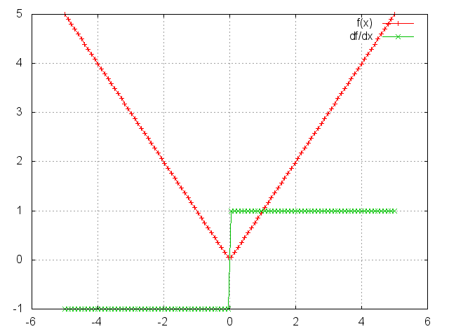
Abs
module = Abs()
m = nn.Abs()
ii = torch.linspace(-5, 5)
oo = m:forward(ii)
go = torch.ones(100)
gi = m:backward(ii, go)
gnuplot.plot({'f(x)', ii, oo, '+-'}, {'df/dx', ii, gi, '+-'})
gnuplot.grid(true)
Add
module = nn.Add(inputDimension, scalar)
Applies a bias term to the incoming data, i.e. yi = x_i + b_i, or if scalar = true then uses a single bias term, yi = x_i + b. So if scalar = true then inputDimension value will be disregarded.
Example:
y = torch.Tensor(5)
mlp = nn.Sequential()
mlp:add(nn.Add(5))

function gradUpdate(mlp, x, y, criterion, learningRate)
   local pred = mlp:forward(x)
   local err = criterion:forward(pred, y)
   local gradCriterion = criterion:backward(pred, y)
   mlp:zeroGradParameters()
   mlp:backward(x, gradCriterion)
   mlp:updateParameters(learningRate)
   return err
end

for i = 1, 10000 do
   x = torch.rand(5)
   y:copy(x);
   for i = 1, 5 do y[i] = y[i] + i; end
   err = gradUpdate(mlp, x, y, nn.MSECriterion(), 0.01)
end

print(mlp:get(1).bias)
gives the output:
 1.0000
 2.0000
 3.0000
 4.0000
 5.0000
[torch.Tensor of dimension 5]
i.e. the network successfully learns the input x has been shifted to produce the output y.
CAdd
module = nn.CAdd(size)
Applies a component-wise addition to the incoming data, i.e. y_i = x_i + b_i. Argument size can be one or many numbers (sizes) or a torch.LongStorage. For example, nn.CAdd(3,4,5) is equivalent to nn.CAdd(torch.LongStorage{3,4,5}). If the size for a particular dimension is 1, the addition will be expanded along the entire axis.
Example:
mlp = nn.Sequential()
mlp:add(nn.CAdd(5, 1))

y = torch.Tensor(5, 4)
bf = torch.Tensor(5, 4)
for i = 1, 5 do bf[i] = i; end -- scale input with this

function gradUpdate(mlp, x, y, criterion, learningRate)
   local pred = mlp:forward(x)
   local err = criterion:forward(pred, y)
   local gradCriterion = criterion:backward(pred, y)
   mlp:zeroGradParameters()
   mlp:backward(x, gradCriterion)
   mlp:updateParameters(learningRate)
   return err
end

for i = 1, 10000 do
   x = torch.rand(5, 4)
   y:copy(x)
   y:add(bf)
   err = gradUpdate(mlp, x, y, nn.MSECriterion(), 0.01)
end

print(mlp:get(1).bias)
gives the output:
 1.0000
 2.0000
 3.0000
 4.0000
 5.0000
[torch.Tensor of dimension 5x1]
i.e. the network successfully learns the input x has been shifted by those bias factors to produce the output y.
Mul
module = nn.Mul()
Applies a single scaling factor to the incoming data, i.e. y = w x, where w is a scalar.
Example:
y = torch.Tensor(5)
mlp = nn.Sequential()
mlp:add(nn.Mul())

function gradUpdate(mlp, x, y, criterion, learningRate)
   local pred = mlp:forward(x)
   local err = criterion:forward(pred, y)
   local gradCriterion = criterion:backward(pred, y)
   mlp:zeroGradParameters()
   mlp:backward(x, gradCriterion)
   mlp:updateParameters(learningRate)
   return err
end

for i = 1, 10000 do
   x = torch.rand(5)
   y:copy(x)
   y:mul(math.pi)
   err = gradUpdate(mlp, x, y, nn.MSECriterion(), 0.01)
end

print(mlp:get(1).weight)
gives the output:
 3.1416
[torch.Tensor of dimension 1]
i.e. the network successfully learns the input x has been scaled by pi.
CMul
module = nn.CMul(size)
Applies a component-wise multiplication to the incoming data, i.e. y_i = w_i * x_i. Argument size can be one or many numbers (sizes) or a torch.LongStorage. For example, nn.CMul(3,4,5) is equivalent to nn.CMul(torch.LongStorage{3,4,5}).
If the size for a particular dimension is 1, the multiplication will be expanded along the entire axis.
Example:
mlp = nn.Sequential()
mlp:add(nn.CMul(5, 1))

y = torch.Tensor(5, 4)
sc = torch.Tensor(5, 4)
for i = 1, 5 do sc[i] = i; end -- scale input with this

function gradUpdate(mlp, x, y, criterion, learningRate)
   local pred = mlp:forward(x)
   local err = criterion:forward(pred, y)
   local gradCriterion = criterion:backward(pred, y)
   mlp:zeroGradParameters()
   mlp:backward(x, gradCriterion)
   mlp:updateParameters(learningRate)
   return err
end

for i = 1, 10000 do
   x = torch.rand(5, 4)
   y:copy(x)
   y:cmul(sc)
   err = gradUpdate(mlp, x, y, nn.MSECriterion(), 0.01)
end

print(mlp:get(1).weight)
gives the output:
 1.0000
 2.0000
 3.0000
 4.0000
 5.0000
[torch.Tensor of dimension 5x1]
i.e. the network successfully learns the input x has been scaled by those scaling factors to produce the output y.
Max
module = nn.Max(dimension, nInputDim)
Applies a max operation over dimension dimension.
Hence, if an nxpxq Tensor was given as input, and dimension = 2 then an nxq matrix would be output.
When nInputDim is provided, inputs larger than that value will be considered batches where the actual dimension to apply the max operation will be dimension dimension + 1.
Min
module = nn.Min(dimension, nInputDim)
Applies a min operation over dimension dimension.
Hence, if an nxpxq Tensor was given as input, and dimension = 2 then an nxq matrix would be output.
When nInputDim is provided, inputs larger than that value will be considered batches where the actual dimension to apply the min operation will be dimension dimension + 1.
Mean
module = nn.Mean(dimension, nInputDim)
Applies a mean operation over dimension dimension.
Hence, if an nxpxq Tensor was given as input, and dimension = 2 then an nxq matrix would be output.
When nInputDim is provided , inputs larger than that value will be considered batches where the actual dimension to apply the sum operation will be dimension dimension + 1.
This module is based on nn.Sum.
Sum
module = nn.Sum(dimension, nInputDim, sizeAverage, squeeze)
Applies a sum operation over dimension dimension.
Hence, if an nxpxq Tensor was given as input, and dimension = 2 then an nxq matrix would be output. If argument squeeze is set to false then the output would be of size nx1xq.
When nInputDim is provided , inputs larger than that value will be considered batches where the actual dimension to apply the sum operation will be dimension dimension + 1.
Negative indexing is allowed by providing a negative value to nInputDim.
When sizeAverage is provided, the sum is divided by the size of the input in this dimension. This is equivalent to the mean operation performed by the nn.Mean module.
Euclidean
module = nn.Euclidean(inputSize,outputSize)
Outputs the Euclidean distance of the input to outputSize centers, i.e. this layer has the weights w_j, for j = 1,..,outputSize, where w_j are vectors of dimension inputSize.
The distance y_j between center j and input x is formulated as y_j = || w_j - x ||.
WeightedEuclidean
module = nn.WeightedEuclidean(inputSize,outputSize)
This module is similar to Euclidean, but additionally learns a separate diagonal covariance matrix across the features of the input space for each center.
In other words, for each of the outputSize centers w_j, there is a diagonal covariance matrices c_j, for j = 1,..,outputSize, where c_j are stored as vectors of size inputSize.
The distance y_j between center j and input x is formulated as y_j = || c_j * (w_j - x) ||.
Cosine
module = nn.Cosine(inputSize,outputSize)
Outputs the cosine similarity of the input to outputSize centers, i.e. this layer has the weights w_j, for j = 1,..,outputSize, where w_j are vectors of dimension inputSize.
The distance y_j between center j and input x is formulated as y_j = (x · w_j) / ( || w_j || * || x || ).
Kmeans
km = nn.Kmeans(k, dim)
k is the number of centroids and dim is the dimensionality of samples.
The forward pass computes distances with respect to centroids and returns index of closest centroid.
Centroids can be updated using gradient descent.
Centroids can be initialized randomly or by using kmeans++ algoirthm:
km:initRandom(samples) -- Randomly initialize centroids from input samples.
km:initKmeansPlus(samples) -- Use Kmeans++ to initialize centroids.
Example showing how to use Kmeans module to do standard Kmeans clustering.
attempts = 10
iter = 100 -- Number of iterations
bestKm = nil
bestLoss = math.huge
learningRate = 1
for j=1, attempts do
   local km = nn.Kmeans(k, dim)
   km:initKmeansPlus(samples)
   for i=1, iter do
      km:zeroGradParameters()
      km:forward(samples) -- sets km.loss
      km:backward(samples, gradOutput) -- gradOutput is ignored

      -- Gradient Descent weight/centroids update
      km:updateParameters(learningRate)
   end

   if km.loss < bestLoss then
      bestLoss = km.loss
      bestKm = km:clone()
   end
end
nn.Kmeans() module maintains loss only for the latest forward. If you want to maintain loss over the whole dataset then you who would need do it my adding the module loss for every forward.
You can also use nn.Kmeans() as an auxillary layer in your network.
A call to forward will generate an output containing the index of the nearest cluster for each sample in the batch.
The gradInput generated by updateGradInput will be zero.
Identity
module = nn.Identity()
Creates a module that returns whatever is input to it as output. This is useful when combined with the module ParallelTable in case you do not wish to do anything to one of the input Tensors.
Example:
mlp = nn.Identity()
print(mlp:forward(torch.ones(5, 2)))
gives the output:
 1  1
 1  1
 1  1
 1  1
 1  1
[torch.Tensor of dimension 5x2]
Here is a more useful example, where one can implement a network which also computes a Criterion using this module:
pred_mlp = nn.Sequential()  -- A network that makes predictions given x.
pred_mlp:add(nn.Linear(5, 4))
pred_mlp:add(nn.Linear(4, 3))

xy_mlp = nn.ParallelTable() -- A network for predictions and for keeping the
xy_mlp:add(pred_mlp)        -- true label for comparison with a criterion
xy_mlp:add(nn.Identity())   -- by forwarding both x and y through the network.

mlp = nn.Sequential()       -- The main network that takes both x and y.
mlp:add(xy_mlp)             -- It feeds x and y to parallel networks;
cr = nn.MSECriterion()
cr_wrap = nn.CriterionTable(cr)
mlp:add(cr_wrap)            -- and then applies the criterion.

for i = 1, 100 do           -- Do a few training iterations
   x = torch.ones(5)        -- Make input features.
   y = torch.Tensor(3)
   y:copy(x:narrow(1,1,3))  -- Make output label.
   err = mlp:forward{x,y}   -- Forward both input and output.
   print(err)               -- Print error from criterion.

   mlp:zeroGradParameters() -- Do backprop...
   mlp:backward({x, y})
   mlp:updateParameters(0.05)
end
Copy
module = nn.Copy(inputType, outputType, [forceCopy, dontCast])
This layer copies the input to output with type casting from inputType to outputType. Unless forceCopy is true, when the first two arguments are the same, the input isn't copied, only transferred as the output.
The default forceCopy is false.
When dontCast is true, a call to nn.Copy:type(type) will not cast the module's output and gradInput Tensors to the new type.
The default is false.
Narrow
module = nn.Narrow(dimension, offset, length)
Narrow is application of narrow operation in a module. The module further supports negative length, dim and offset to handle inputs of unknown size.
> x = torch.rand(4, 5)

> x
 0.3695  0.2017  0.4485  0.4638  0.0513
 0.9222  0.1877  0.3388  0.6265  0.5659
 0.8785  0.7394  0.8265  0.9212  0.0129
 0.2290  0.7971  0.2113  0.1097  0.3166
[torch.DoubleTensor of size 4x5]

> nn.Narrow(1, 2, 3):forward(x)
 0.9222  0.1877  0.3388  0.6265  0.5659
 0.8785  0.7394  0.8265  0.9212  0.0129
 0.2290  0.7971  0.2113  0.1097  0.3166
[torch.DoubleTensor of size 3x5]

> nn.Narrow(1, 2, -1):forward(x)
 0.9222  0.1877  0.3388  0.6265  0.5659
 0.8785  0.7394  0.8265  0.9212  0.0129
 0.2290  0.7971  0.2113  0.1097  0.3166
[torch.DoubleTensor of size 3x5]

> nn.Narrow(1, 2, 2):forward(x)
 0.9222  0.1877  0.3388  0.6265  0.5659
 0.8785  0.7394  0.8265  0.9212  0.0129
[torch.DoubleTensor of size 2x5]

> nn.Narrow(1, 2, -2):forward(x)
 0.9222  0.1877  0.3388  0.6265  0.5659
 0.8785  0.7394  0.8265  0.9212  0.0129
[torch.DoubleTensor of size 2x5]

> nn.Narrow(2, 2, 3):forward(x)
 0.2017  0.4485  0.4638
 0.1877  0.3388  0.6265
 0.7394  0.8265  0.9212
 0.7971  0.2113  0.1097
[torch.DoubleTensor of size 4x3]

> nn.Narrow(2, 2, -2):forward(x)
 0.2017  0.4485  0.4638
 0.1877  0.3388  0.6265
 0.7394  0.8265  0.9212
 0.7971  0.2113  0.1097
[torch.DoubleTensor of size 4x3]
Replicate
module = nn.Replicate(nFeature [, dim, ndim])
This class creates an output where the input is replicated nFeature times along dimension dim (default 1).
There is no memory allocation or memory copy in this module.
It sets the stride along the dimth dimension to zero.
When provided, ndim should specify the number of non-batch dimensions.
This allows the module to replicate the same non-batch dimension dim for both batch and non-batch inputs.
> x = torch.linspace(1, 5, 5)
 1
 2
 3
 4
 5
[torch.DoubleTensor of dimension 5]

> m = nn.Replicate(3)
> o = m:forward(x)
 1  2  3  4  5
 1  2  3  4  5
 1  2  3  4  5
[torch.DoubleTensor of dimension 3x5]

> x:fill(13)
 13
 13
 13
 13
 13
[torch.DoubleTensor of dimension 5]

> print(o)
 13  13  13  13  13
 13  13  13  13  13
 13  13  13  13  13
[torch.DoubleTensor of dimension 3x5]
Reshape
module = nn.Reshape(dimension1, dimension2, ... [, batchMode])
Reshapes an nxpxqx.. Tensor into a dimension1xdimension2x... Tensor, taking the elements row-wise.
The optional last argument batchMode, when true forces the first dimension of the input to be considered the batch dimension, and thus keep its size fixed.
This is necessary when dealing with batch sizes of one.
When false, it forces the entire input (including the first dimension) to be reshaped to the input size.
Default batchMode=nil, which means that the module considers inputs with more elements than the produce of provided sizes, i.e. dimension1xdimension2x..., to be batches.
Example:
> x = torch.Tensor(4,4)
> for i = 1, 4 do
>    for j = 1, 4 do
>       x[i][j] = (i-1)*4+j
>    end
> end
> print(x)

  1   2   3   4
  5   6   7   8
  9  10  11  12
 13  14  15  16
[torch.Tensor of dimension 4x4]

> print(nn.Reshape(2,8):forward(x))

  1   2   3   4   5   6   7   8
  9  10  11  12  13  14  15  16
[torch.Tensor of dimension 2x8]

> print(nn.Reshape(8,2):forward(x))

  1   2
  3   4
  5   6
  7   8
  9  10
 11  12
 13  14
 15  16
[torch.Tensor of dimension 8x2]

> print(nn.Reshape(16):forward(x))

  1
  2
  3
  4
  5
  6
  7
  8
  9
 10
 11
 12
 13
 14
 15
 16
[torch.Tensor of dimension 16]

> y = torch.Tensor(1, 4):fill(0)
> print(y)

 0  0  0  0
 [torch.DoubleTensor of dimension 1x4]

> print(nn.Reshape(4):forward(y))

 0  0  0  0
 [torch.DoubleTensor of dimension 1x4]

> print(nn.Reshape(4, false):forward(y))

 0
 0
 0
 0
 [torch.DoubleTensor of dimension 4]
View
module = nn.View(sizes)
This module creates a new view of the input tensor using the sizes passed to the constructor. The parameter sizes can either be a LongStorage or numbers.
The method setNumInputDims() allows to specify the expected number of dimensions of the inputs of the modules.
This makes it possible to use minibatch inputs when using a size -1 for one of the dimensions.
The method resetSize(sizes) allows to reset the view size of the module after initialization.
Example 1:
> x = torch.Tensor(4, 4)
> for i = 1, 4 do
>    for j = 1, 4 do
>       x[i][j] = (i-1)*4+j
>    end
> end
> print(x)

  1   2   3   4
  5   6   7   8
  9  10  11  12
 13  14  15  16
[torch.Tensor of dimension 4x4]

> print(nn.View(2, 8):forward(x))

  1   2   3   4   5   6   7   8
  9  10  11  12  13  14  15  16
[torch.DoubleTensor of dimension 2x8]

> print(nn.View(torch.LongStorage{8,2}):forward(x))

  1   2
  3   4
  5   6
  7   8
  9  10
 11  12
 13  14
 15  16
[torch.DoubleTensor of dimension 8x2]

> print(nn.View(16):forward(x))

  1
  2
  3
  4
  5
  6
  7
  8
  9
 10
 11
 12
 13
 14
 15
 16
[torch.DoubleTensor of dimension 16]
Example 2:
> input = torch.Tensor(2, 3)
> minibatch = torch.Tensor(5, 2, 3)
> m = nn.View(-1):setNumInputDims(2)
> print(#m:forward(input))

 6
[torch.LongStorage of size 1]

> print(#m:forward(minibatch))

 5
 6
[torch.LongStorage of size 2]
For collapsing non-batch dims, check out nn.Collapse.
Contiguous
module = nn.Contiguous()
Is used to make input, gradOutput or both contiguous, corresponds to torch.contiguous function.
Only does copy and allocation if input or gradOutput is not contiguous, otherwise passes the same Tensor.
Select
module = nn.Select(dim, index)
Selects a dimension and index of a nxpxqx.. Tensor.
Example:
mlp = nn.Sequential()
mlp:add(nn.Select(1, 3))

x = torch.randn(10, 5)
print(x)
print(mlp:forward(x))
gives the output:
 0.9720 -0.0836  0.0831 -0.2059 -0.0871
 0.8750 -2.0432 -0.1295 -2.3932  0.8168
 0.0369  1.1633  0.6483  1.2862  0.6596
 0.1667 -0.5704 -0.7303  0.3697 -2.2941
 0.4794  2.0636  0.3502  0.3560 -0.5500
-0.1898 -1.1547  0.1145 -1.1399  0.1711
-1.5130  1.4445  0.2356 -0.5393 -0.6222
-0.6587  0.4314  1.1916 -1.4509  1.9400
 0.2733  1.0911  0.7667  0.4002  0.1646
 0.5804 -0.5333  1.1621  1.5683 -0.1978
[torch.Tensor of dimension 10x5]

 0.0369
 1.1633
 0.6483
 1.2862
 0.6596
[torch.Tensor of dimension 5]
This can be used in conjunction with Concat to emulate the behavior of Parallel, or to select various parts of an input Tensor to perform operations on. Here is a fairly complicated example:
mlp = nn.Sequential()
c = nn.Concat(2)
for i = 1, 10 do
   local t = nn.Sequential()
   t:add(nn.Select(1, i))
   t:add(nn.Linear(3, 2))
   t:add(nn.Reshape(2, 1))
   c:add(t)
end
mlp:add(c)

pred = mlp:forward(torch.randn(10, 3))
print(pred)

for i = 1, 10000 do     -- Train for a few iterations
   x = torch.randn(10, 3)
   y = torch.ones(2, 10)
   pred = mlp:forward(x)

   criterion = nn.MSECriterion()
   err = criterion:forward(pred, y)
   gradCriterion = criterion:backward(pred, y)
   mlp:zeroGradParameters()
   mlp:backward(x, gradCriterion)
   mlp:updateParameters(0.01)
   print(err)
end
MaskedSelect
module = nn.MaskedSelect()
Performs a torch.MaskedSelect on a Tensor.
The mask is supplied as a tabular argument with the input on the forward and backward passes.
Example:
ms = nn.MaskedSelect()
mask = torch.ByteTensor({{1, 0}, {0, 1}})
input = torch.DoubleTensor({{10, 20}, {30, 40}})
print(input)
print(mask)
out = ms:forward({input, mask})
print(out)
gradIn = ms:backward({input, mask}, out)
print(gradIn[1])
Gives the output:
10  20
30  40
[torch.DoubleTensor of size 2x2]

1  0
0  1
[torch.ByteTensor of size 2x2]

10
40
[torch.DoubleTensor of size 2]

10  0
0  40
[torch.DoubleTensor of size 2x2]
Index
module = nn.Index(dim)
Applies the Tensor index operation along the given dimension. So
nn.Index(dim):forward{t,i}
gives the same output as
t:index(dim, i)
Squeeze
module = nn.Squeeze([dim, numInputDims])
Applies the Tensor squeeze operation. So
nn.Squeeze():forward(t)
gives the same output as
t:squeeze()
Setting numInputDims allows to use this module on batches.
Unsqueeze
module = nn.Unsqueeze(pos [, numInputDims])
Insert singleton dim (i.e., dimension 1) at position pos.
For an input with dim = input:dim(), there are dim + 1 possible positions to insert the singleton dimension.
For example, if input is 3 dimensional Tensor in size p x q x r, then the singleton dim can be inserted at the following 4 positions
pos = 1: 1 x p x q x r
pos = 2: p x 1 x q x r
pos = 3: p x q x 1 x r
pos = 4: p x q x r x 1
Example:
input = torch.Tensor(2, 4, 3) -- input: 2 x 4 x 3

-- insert at head
m = nn.Unsqueeze(1)
m:forward(input) -- output: 1 x 2 x 4 x 3

-- insert at tail
m = nn.Unsqueeze(4)
m:forward(input) -- output: 2 x 4 x 3 x 1

-- insert in between
m = nn.Unsqueeze(2)
m:forward(input) -- output: 2 x 1 x 4 x 3

-- the input size can vary across calls
input2 = torch.Tensor(3, 5, 7) -- input2: 3 x 5 x 7
m:forward(input2) -- output: 3 x 1 x 5 x 7
Indicate the expected input feature map dimension by specifying numInputDims.
This allows the module to work with mini-batch. Example:
b = 5 -- batch size 5
input = torch.Tensor(b, 2, 4, 3) -- input: b x 2 x 4 x 3
numInputDims = 3 -- input feature map should be the last 3 dims

m = nn.Unsqueeze(4, numInputDims)
m:forward(input) -- output: b x 2 x 4 x 3 x 1

m = nn.Unsqueeze(2):setNumInputDims(numInputDims)
m:forward(input) -- output: b x 2 x 1 x 4 x 3
Transpose
module = nn.Transpose({dim1, dim2} [, {dim3, dim4}, ...])
Swaps dimension dim1 with dim2, then dim3 with dim4, and so on. So
nn.Transpose({dim1, dim2}, {dim3, dim4}):forward(t)
gives the same output as
t:transpose(dim1, dim2)
t:transpose(dim3, dim4)
The method setNumInputDims() allows to specify the expected number of dimensions of the inputs of the modules. This makes it possible to use minibatch inputs. Example:
b = 5 -- batch size 5
input = torch.Tensor(b, 2, 4, 3) -- input: b x 2 x 4 x 3

m = nn.Transpose({1,3})
m:forward(input) -- output: 4 x 2 x b x 3 x 1

numInputDims = 3 -- input feature map should be the last 3 dims
m = nn.Transpose({1,3}):setNumInputDims(numInputDims)
m:forward(input) -- output: b x 3 x 4 x 2
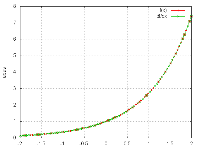
Exp
module = nn.Exp()
Applies the exp function element-wise to the input Tensor, thus outputting a Tensor of the same dimension.
ii = torch.linspace(-2, 2)
m = nn.Exp()
oo = m:forward(ii)
go = torch.ones(100)
gi = m:backward(ii,go)
gnuplot.plot({'f(x)', ii, oo, '+-'}, {'df/dx', ii, gi, '+-'})
gnuplot.grid(true)
Log
module = nn.Log()
Applies the log function element-wise to the input Tensor, thus outputting a Tensor of the same dimension.
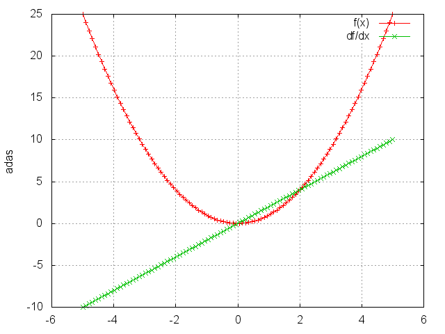
Square
module = nn.Square()
Takes the square of each element.
ii = torch.linspace(-5, 5)
m = nn.Square()
oo = m:forward(ii)
go = torch.ones(100)
gi = m:backward(ii, go)
gnuplot.plot({'f(x)', ii, oo, '+-'}, {'df/dx', ii, gi, '+-'})
gnuplot.grid(true)
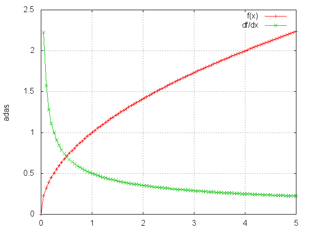
Sqrt
module = nn.Sqrt()
Takes the square root of each element.
ii = torch.linspace(0, 5)
m = nn.Sqrt()
oo = m:forward(ii)
go = torch.ones(100)
gi = m:backward(ii, go)
gnuplot.plot({'f(x)', ii, oo, '+-'}, {'df/dx', ii, gi, '+-'})
gnuplot.grid(true)
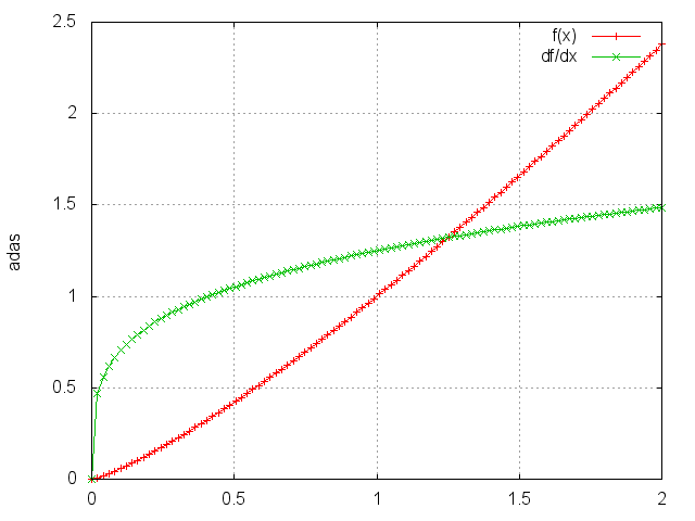
Power
module = nn.Power(p)
Raises each element to its p-th power.
ii = torch.linspace(0, 2)
m = nn.Power(1.25)
oo = m:forward(ii)
go = torch.ones(100)
gi = m:backward(ii, go)
gnuplot.plot({'f(x)', ii, oo, '+-'}, {'df/dx', ii, gi, '+-'})
gnuplot.grid(true)
Clamp
module = nn.Clamp(min_value, max_value)
Clamps all elements into the range [min_value, max_value].
Output is identical to input in the range, otherwise elements less than min_value (or greater than max_value) are saturated to min_value (or max_value).
A = torch.randn(2, 5)
m = nn.Clamp(-0.1, 0.5)
B = m:forward(A)

print(A)  -- input
-1.1321  0.0227 -0.4672  0.6519 -0.5380
 0.9061 -1.0858  0.3697 -0.8120 -1.6759
[torch.DoubleTensor of size 3x5]

print(B)  -- output
-0.1000  0.0227 -0.1000  0.5000 -0.1000
 0.5000 -0.1000  0.3697 -0.1000 -0.1000
[torch.DoubleTensor of size 3x5]
Normalize
module = nn.Normalize(p, [eps])
Normalizes the input Tensor to have unit L_p norm. The smoothing parameter eps prevents division by zero when the input contains all zero elements (default = 1e-10).
Input can be 1D or 2D (in which case it's considered as in batch mode)
A = torch.randn(3, 5)
m = nn.Normalize(2)
B = m:forward(A) -- B is also 3 x 5
-- take the L2 norm over the second axis:
print(torch.norm(B, 2, 2)) -- norms is [1, 1, 1]
Normalize has a specialized implementation for the inf norm, which corresponds to the maximum norm.
A = torch.randn(3,5)
m = nn.Normalize(math.huge) -- uses maximum/inf norm
B = m:forward(A)
maxA = torch.abs(A):max(2)
print(A,B,maxA)
MM
module = nn.MM(transA, transB)
Performs multiplications on one or more pairs of matrices. If transA is set to true, the first matrix is transposed before multiplication. If transB is set to true, the second matrix is transposed before multiplication. By default, the matrices do not get transposed.
The module also accepts 3D inputs which are interpreted as batches of matrices. When using batches, the first input matrix should be of size b x m x n and the second input matrix should be of size b x n x p (assuming transA and transB are not set). If transA or transB is set, transpose takes place between the second and the third dimensions for the corresponding matrix.
model = nn.MM()
A = torch.randn(b, m, n)
B = torch.randn(b, n, p)
C = model:forward({A, B})  -- C will be of size `b x m x p`

model = nn.MM(true, false)
A = torch.randn(b, n, m)
B = torch.randn(b, n, p)
C = model:forward({A, B})  -- C will be of size `b x m x p`
BatchNormalization
module = nn.BatchNormalization(N [, eps] [, momentum] [,affine])
where N is the dimensionality of input
eps is a small value added to the standard-deviation to avoid divide-by-zero. Defaults to 1e-5.
affine is a boolean. When set to false, the learnable affine transform is disabled. Defaults to true
During training, this layer keeps a running estimate of its computed mean and std. The running sum is kept with a default momentum of 0.1 (unless over-ridden) During evaluation, this running mean/std is used for normalization.
Implements Batch Normalization as described in the paper: "Batch Normalization: Accelerating Deep Network Training by Reducing Internal Covariate Shift" by Sergey Ioffe, Christian Szegedy.
The operation implemented is:
              x - mean(x)
y =  ----------------------------- * gamma + beta
      standard-deviation(x) + eps
where the mean and standard-deviation are calculated per-dimension over the mini-batches and where gamma and beta are learnable parameter vectors of size N (where N is the input size).
The learning of gamma and beta is optional.
The module only accepts 2D inputs.
-- with learnable parameters
model = nn.BatchNormalization(m)
A = torch.randn(b, m)
C = model:forward(A)  -- C will be of size `b x m`

-- without learnable parameters
model = nn.BatchNormalization(m, nil, nil, false)
A = torch.randn(b, m)
C = model:forward(A)  -- C will be of size `b x m`
PixelShuffle
module = nn.PixelShuffle(r)
Rearranges elements in a tensor of shape [C*r*r, H, W] to a tensor of shape [C, H*r, W*r]. This is useful for implementing efficient sub-pixel convolution with a stride of 1/r (see Shi et. al). Below we show how the PixelShuffle module can be used to learn upscaling filters to transform a low-resolution input to a high resolution one, with a 3x upscale factor. This is useful for tasks such as super-resolution, see "Real-Time Single Image and Video Super-Resolution Using an Efficient Sub-Pixel Convolutional Neural Network" - Shi et al. for further details.
upscaleFactor = 3
inputChannels = 1

model = nn.Sequential()
model:add(nn.SpatialConvolution(inputChannels, 64, 5, 5, 1, 1, 2, 2))
model:add(nn.ReLU())

model:add(nn.SpatialConvolution(64, 32, 3, 3, 1, 1, 1, 1))
model:add(nn.ReLU())

model:add(nn.SpatialConvolution(32, inputChannels * upscaleFactor * upscaleFactor, 3, 3, 1, 1, 1, 1))
model:add(nn.PixelShuffle(upscaleFactor))

input = torch.Tensor(1, 192, 256);
out = model:forward(input)
out:size()
   1
 576
 768
[torch.LongStorage of size 3]
Padding
module = nn.Padding(dim, pad [, nInputDim, value, index])
This module adds pad units of padding to dimension dim of the input.
If pad is negative, padding is added to the left, otherwise, it is added to the right of the dimension. When nInputDim is provided, inputs larger than that value will be considered batches where the actual dim to be padded will
be dimension dim + 1. When value is provide, the padding will be filled with that value. The default value is zero.
When index is provided, padding will be added at that offset from the left or right, depending on the sign of pad.
Example 1:
module = nn.Padding(1, 2, 1, -1) --pad right x2
module:forward(torch.randn(3)) --non-batch input
 0.2008
 0.4848
-1.0783
-1.0000
-1.0000
[torch.DoubleTensor of dimension 5]
Example 2:
module = nn.Padding(1, -2, 1, -1) --pad left x2
module:forward(torch.randn(2, 3)) --batch input
-1.0000 -1.0000  1.0203  0.2704 -1.6164
-1.0000 -1.0000 -0.2219 -0.6529 -1.9218
[torch.DoubleTensor of dimension 2x5]
Example 3:
module = nn.Padding(1, -2, 1, -1, 2) --pad left x2, offset to index 2
module:forward(torch.randn(2, 3)) --batch input
 1.0203 -1.0000 -1.0000  0.2704 -1.6164
-0.6529 -1.0000 -1.0000 -0.2219 -1.9218
[torch.DoubleTensor of dimension 2x5]
L1Penalty
penalty = nn.L1Penalty(L1weight, sizeAverage)
L1Penalty is an inline module that in its forward propagation copies the input Tensor directly to the output, and computes an L1 loss of the latent state (input) and stores it in the module's loss field.
During backward propagation: gradInput = gradOutput + gradLoss.
This module can be used in autoencoder architectures to apply L1 losses to internal latent state without having to use Identity and parallel containers to carry the internal code to an output criterion.
Example (sparse autoencoder, note: decoder should be normalized):
encoder = nn.Sequential()
encoder:add(nn.Linear(3, 128))
encoder:add(nn.Threshold())
decoder = nn.Linear(128, 3)

autoencoder = nn.Sequential()
autoencoder:add(encoder)
autoencoder:add(nn.L1Penalty(l1weight))
autoencoder:add(decoder)

criterion = nn.MSECriterion()  -- To measure reconstruction error
-- ...
GradientReversal
module = nn.GradientReversal([lambda = 1])
This module preserves the input, but takes the gradient from the subsequent layer, multiplies it by -lambda and passes it to the preceding layer. This can be used to maximise an objective function whilst using gradient descent, as described in "Domain-Adversarial Training of Neural Networks" (http://arxiv.org/abs/1505.07818).
One can also call:
module:setLambda(lambda)
to set the hyper-parameter lambda dynamically during training.
GPU
gpu = nn.GPU(module, device, [outdevice])
require 'cunn'
gpu:cuda()
Decorates an encapsulated module so that it can be executed on a specific GPU device.
The decorated module's parameters are thus hosted on the specified GPU device.
All operations on the gpu module are executed on that device.
Calls to forward/backward will transfer arguments input and gradOutput to the specified device,
which are then fed as arguments to the decorated module.
Returned output is located on the specified outdevice (defaults to device).
Returned gradInput is allocated on the same device as the input.
When serialized/deserialized, the gpu module will be run on the same device that it was serialized with.
To prevent this from happening, the module can be converted to float/double before serialization:
gpu:float()
gpustr = torch.serialize(gpu)
The module is located in the nn package instead of cunn as this allows it to be used in CPU-only environments, which are common for production models.
The module supports nested table input and gradOutput tensors originating from multiple devices.
Each nested tensor in the returned gradInput will be transferred to the device its commensurate tensor in the input.
The intended use-case is not for model-parallelism where the models are executed in parallel on multiple devices, but for sequential models where a single GPU doesn't have enough memory.
Example using 4 GPUs:
mlp = nn.Sequential()
   :add(nn.GPU(nn.Linear(10000,10000), 1))
   :add(nn.GPU(nn.Linear(10000,10000), 2))
   :add(nn.GPU(nn.Linear(10000,10000), 3))
   :add(nn.GPU(nn.Linear(10000,10000), 4, cutorch.getDevice()))
Note how the last GPU instance will return an output tensor on the same device as the current device (cutorch.getDevice).
TemporalDynamicKMaxPooling
module = nn.TemporalDynamicKMaxPooling(minK, [factor])
Selects the highest k values for each feature in the feature map sequence provided. The input sequence is composed of nInputFrame frames (i.e. nInputFrame is sequence length). The input tensor in forward(input) is expected to be a 2D tensor (nInputFrame x inputFrameSize) or a 3D tensor (nBatchFrame x nInputFrame x inputFrameSize), where inputFrameSize is the number of features across the sequence.
If factor is not provided, k = minK, else the value of k is calculated with:
k = math.max(minK, math.ceil(factor*nInputFrame)))
Constant
module = nn.Constant(value, nInputDim)
This module outputs a constant value given an input.
If nInputDim is specified, it uses the input to determine the size of the batch.
The value is then replicated over the batch.
Otherwise, the value Tensor is output as is.
During backward, the returned gradInput is a zero Tensor of the same size as the input.
This module has no trainable parameters.
You can use this with nn.ConcatTable() to append constant inputs to an input :
nn.ConcatTable():add(nn.Constant(v)):add(nn.Identity())
This is useful when you want to output a value that is independent of the input to the neural network.
WhiteNoise
module = nn.WhiteNoise([mean, stdev])
This module adds isotropic Gaussian noise to the input.
This can be useful for training Denoising Autoencoders.
Takes mean and stdev of the normal distribution as constructor arguments.
Default values for mean and standard deviation are 0 and 0.1 respectively.
With module:training(), Gaussian noise is added during forward.
During backward gradients are passed as is.
With module:evaluate() the mean is added to the input.
OneHot
module = nn.OneHot(outputSize)
Transforms a tensor of input indices having integer values between 1 and outputSize into
a tensor of one-hot vectors of size outputSize.
Forward an index to get a one-hot vector :
> module = nn.OneHot(5) -- 5 classes
> module:forward(torch.LongTensor{3})
 0  0  1  0  0
[torch.DoubleTensor of size 1x5]
Forward a batch of 3 indices. Notice that these need not be stored as torch.LongTensor :
> module:forward(torch.Tensor{3,2,1})
 0  0  1  0  0
 0  1  0  0  0
 1  0  0  0  0
[torch.DoubleTensor of size 3x5]
Forward batch of 2 x 3 indices :
oh:forward(torch.Tensor{{3,2,1},{1,2,3}})
(1,.,.) =
  0  0  1  0  0
  0  1  0  0  0
  1  0  0  0  0

(2,.,.) =
  1  0  0  0  0
  0  1  0  0  0
  0  0  1  0  0
[torch.DoubleTensor of size 2x3x5]
PrintSize
module = nn.PrintSize(name)
This module is useful for debugging complicated module composites.
It prints the size of the input and gradOutput during forward
and backward propagation respectively.
The name is a string used to identify the module along side the printed size.
ZeroGrad
module = nn.ZeroGrad()
input = torch.Tensor{1,2}
gradOutput = torch.Tensor{3,4}
print(module:forward(input))
 1
 2
[torch.DoubleTensor of size 2]

print(module:backward(input, gradOutput))
 0
 0
[torch.DoubleTensor of size 2]
The module zeros the gradInput but forwards the input as-is.
Collapse
module = nn.Collapse(nInputDim)
This module is the equivalent of:
view = nn.View(-1)
view:setNumInputDim(nInputDim)
It collapses all non-batch dimensions. This is useful for converting a spatial feature map to the single dimension required by a dense hidden layer like Linear.
Convert
module = nn.Convert([inputShape, outputShape])
Module to convert between different data formats. For example, we can flatten images by using :
module = nn.Convert('bchw', 'bf')
or equivalently
module = nn.Convert('chw', 'f')
Lets try it with an input:
print(module:forward(torch.randn(3,2,3,1)))
 0.5692 -0.0190  0.5243  0.7530  0.4230  1.2483
-0.9142  0.6013  0.5608 -1.0417 -1.4014  1.0177
-1.5207 -0.1641 -0.4166  1.4810 -1.1725 -1.0037
[torch.DoubleTensor of size 3x6]
You could also try:
module = nn.Convert('chw', 'hwc')
input = torch.randn(1,2,3,2)
input:select(2,1):fill(1)
input:select(2,2):fill(2)
print(input)
(1,1,.,.) =
  1  1
  1  1
  1  1
(1,2,.,.) =
  2  2
  2  2
  2  2
[torch.DoubleTensor of size 1x2x3x2]
print(module:forward(input))
(1,1,.,.) =
  1  2
  1  2

(1,2,.,.) =
  1  2
  1  2

(1,3,.,.) =
  1  2
  1  2
[torch.DoubleTensor of size 1x3x2x2]
Furthermore, it automatically converts the input to have the same type as self.output
(i.e. the type of the module).
So you can also just use is for automatic input type converions:
module = nn.Convert()
print(module.output) -- type of module
[torch.DoubleTensor with no dimension]
input = torch.FloatTensor{1,2,3}
print(module:forward(input))
 1
 2
 3
[torch.DoubleTensor of size 3]