Convolutional layers
A convolution is an integral that expresses the amount of overlap of one function g as it is shifted over another function f. It therefore "blends" one function with another. The neural network package supports convolution, pooling, subsampling and other relevant facilities. These are divided base on the dimensionality of the input and output Tensors:
- Temporal Modules apply to sequences with a one-dimensional relationship (e.g. sequences of words, phonemes and letters. Strings of some kind).
- TemporalConvolution : a 1D convolution over an input sequence ;
- TemporalSubSampling : a 1D sub-sampling over an input sequence ;
- TemporalMaxPooling : a 1D max-pooling operation over an input sequence ;
- LookupTable : a convolution of width
1, commonly used for word embeddings ;
- Spatial Modules apply to inputs with two-dimensional relationships (e.g. images):
- SpatialConvolution : a 2D convolution over an input image ;
- SpatialSubSampling : a 2D sub-sampling over an input image ;
- SpatialMaxPooling : a 2D max-pooling operation over an input image ;
- SpatialAveragePooling : a 2D average-pooling operation over an input image ;
- SpatialAdaptiveMaxPooling : a 2D max-pooling operation which adapts its parameters dynamically such that the output is of fixed size ;
- SpatialLPPooling : computes the
pnorm in a convolutional manner on a set of input images ; - SpatialConvolutionMap : a 2D convolution that uses a generic connection table ;
- SpatialZeroPadding : padds a feature map with specified number of zeros ;
- SpatialSubtractiveNormalization : a spatial subtraction operation on a series of 2D inputs using a kernel for computing the weighted average in a neighborhood ;
- Volumetric Modules apply to inputs with three-dimensional relationships (e.g. videos) :
- VolumetricConvolution : a 3D convolution over an input video (a sequence of images) ;
- VolumetricMaxPooling : a 3D max-pooling operation over an input video.
Temporal Modules
Excluding and optional first batch dimension, temporal layers expect a 2D Tensor as input. The
first dimension is the number of frames in the sequence (e.g. nInputFrame), the last dimenstion
is the number of features per frame (e.g. inputFrameSize). The output will normally have the same number
of dimensions, although the size of each dimension may change. These are commonly used for processing acoustic signals or sequences of words, i.e. in Natural Language Processing.
Note: The LookupTable is special in that while it does output a temporal Tensor of size nOutputFrame x outputFrameSize,
its input is a 1D Tensor of indices of size nIndices. Again, this is excluding the option first batch dimension.
TemporalConvolution
module = nn.TemporalConvolution(inputFrameSize, outputFrameSize, kW, [dW])
Applies a 1D convolution over an input sequence composed of nInputFrame frames. The input tensor in
forward(input) is expected to be a 2D tensor (nInputFrame x inputFrameSize) or a 3D tensor (nBatchFrame x nInputFrame x inputFrameSize).
The parameters are the following:
* inputFrameSize: The input frame size expected in sequences given into forward().
* outputFrameSize: The output frame size the convolution layer will produce.
* kW: The kernel width of the convolution
* dW: The step of the convolution. Default is 1.
Note that depending of the size of your kernel, several (of the last) frames of the sequence might be lost. It is up to the user to add proper padding frames in the input sequences.
If the input sequence is a 2D tensor of dimension nInputFrame x inputFrameSize, the output sequence will be
nOutputFrame x outputFrameSize where
nOutputFrame = (nInputFrame - kW) / dW + 1
If the input sequence is a 3D tensor of dimension nBatchFrame x nInputFrame x inputFrameSize, the output sequence will be
nBatchFrame x nOutputFrame x outputFrameSize.
The parameters of the convolution can be found in self.weight (Tensor of
size outputFrameSize x (inputFrameSize x kW)) and self.bias (Tensor of
size outputFrameSize). The corresponding gradients can be found in
self.gradWeight and self.gradBias.
For a 2D input, the output value of the layer can be precisely described as:
output[t][i] = bias[i]
  + sum_j sum_{k=1}^kW weight[i][j][k]
                                * input[dW*(t-1)+k)][j]
Here is a simple example:
inp=5;  -- dimensionality of one sequence element
outp=1; -- number of derived features for one sequence element
kw=1;   -- kernel only operates on one sequence element per step
dw=1;   -- we step once and go on to the next sequence element

mlp=nn.TemporalConvolution(inp,outp,kw,dw)

x=torch.rand(7,inp) -- a sequence of 7 elements
print(mlp:forward(x))
which gives:
-0.9109
-0.9872
-0.6808
-0.9403
-0.9680
-0.6901
-0.6387
[torch.Tensor of dimension 7x1]
This is equivalent to:
weights=torch.reshape(mlp.weight,inp) -- weights applied to all
bias= mlp.bias[1];
for i=1,x:size(1) do -- for each sequence element
  element= x[i]; -- features of ith sequence element
  print(element:dot(weights) + bias)
end
which gives:
-0.91094998687717
-0.98721705771773
-0.68075004276185
-0.94030132495887
-0.96798754116609
-0.69008470895581
-0.63871422284166
TemporalMaxPooling
module = nn.TemporalMaxPooling(kW, [dW])
Applies 1D max-pooling operation in kW regions by step size
dW steps. Input sequence composed of nInputFrame frames. The input tensor in
forward(input) is expected to be a 2D tensor (nInputFrame x inputFrameSize)
or a 3D tensor (nBatchFrame x nInputFrame x inputFrameSize).
If the input sequence is a 2D tensor of dimension nInputFrame x inputFrameSize, the output sequence will be
nOutputFrame x inputFrameSize where
nOutputFrame = (nInputFrame - kW) / dW + 1
TemporalSubSampling
module = nn.TemporalSubSampling(inputFrameSize, kW, [dW])
Applies a 1D sub-sampling over an input sequence composed of nInputFrame frames. The input tensor in
forward(input) is expected to be a 2D tensor (nInputFrame x inputFrameSize). The output frame size
will be the same as the input one (inputFrameSize).
The parameters are the following:
* inputFrameSize: The input frame size expected in sequences given into forward().
* kW: The kernel width of the sub-sampling
* dW: The step of the sub-sampling. Default is 1.
Note that depending of the size of your kernel, several (of the last) frames of the sequence might be lost. It is up to the user to add proper padding frames in the input sequences.
If the input sequence is a 2D tensor nInputFrame x inputFrameSize, the output sequence will be
inputFrameSize x nOutputFrame where
nOutputFrame = (nInputFrame - kW) / dW + 1
The parameters of the sub-sampling can be found in self.weight (Tensor of
size inputFrameSize) and self.bias (Tensor of
size inputFrameSize). The corresponding gradients can be found in
self.gradWeight and self.gradBias.
The output value of the layer can be precisely described as:
output[i][t] = bias[i] + weight[i] * sum_{k=1}^kW input[i][dW*(t-1)+k)]
LookupTable
module = nn.LookupTable(nIndex, sizes)
or
module = nn.LookupTable(nIndex, size1, [size2], [size3], ...)
This layer is a particular case of a convolution, where the width of the convolution would be 1.
When calling forward(input), it assumes input is a 1D or 2D tensor filled with indices.
If the input is a matrix, then each row is assumed to be an input sample of given batch. Indices start
at 1 and can go up to nIndex. For each index, it outputs a corresponding Tensor of size
specified by sizes (a LongStorage) or size1 x size2 x....
Given a 1D input, the output tensors are concatenated,
generating a n x size1 x size2 x ... x sizeN tensor, where n
is the size of a 1D input tensor.
Again with a 1D input, when only size1 is provided, the forward(input) is equivalent to
performing the following matrix-matrix multiplication in an efficient manner:
M P
where M is a 2D matrix size1 x nIndex containing the parameters of the lookup-table and
P is a 2D matrix, where each column vector i is a zero vector except at index input[i] where it is 1.
1D example:
 -- a lookup table containing 10 tensors of size 3
 module = nn.LookupTable(10, 3)

 input = torch.Tensor{1,2,1,10}
 print(module:forward(input))
Outputs something like:
-1.4415 -0.1001 -0.1708
-0.6945 -0.4350  0.7977
-1.4415 -0.1001 -0.1708
-0.0745  1.9275  1.0915
[torch.DoubleTensor of dimension 4x3]
Note that the first row vector is the same as the 3rd one!
Given a 2D input tensor of size m x n, the output is a m x n x size1 x size2 x ... x sizeN
tensor, where m is the number of samples in
the batch and n is the number of indices per sample.
2D example:
 -- a lookup table containing 10 tensors of size 3
 module = nn.LookupTable(10, 3)

 -- a batch of 2 samples of 4 indices each
 input = torch.Tensor({{1,2,4,5},{4,3,2,10}})
 print(module:forward(input))
Outputs something like:
(1,.,.) =
 -0.0570 -1.5354  1.8555
 -0.9067  1.3392  0.6275
  1.9662  0.4645 -0.8111
  0.1103  1.7811  1.5969

(2,.,.) =
  1.9662  0.4645 -0.8111
  0.0026 -1.4547 -0.5154
 -0.9067  1.3392  0.6275
 -0.0193 -0.8641  0.7396
[torch.DoubleTensor of dimension 2x4x3]
Spatial Modules
Excluding and optional batch dimension, spatial layers expect a 3D Tensor as input. The
first dimension is the number of features (e.g. frameSize), the last two dimenstions
are spatial (e.g. height x width). These are commonly used for processing images.
SpatialConvolution
module = nn.SpatialConvolution(nInputPlane, nOutputPlane, kW, kH, [dW], [dH])
Applies a 2D convolution over an input image composed of several input planes. The input tensor in
forward(input) is expected to be a 3D tensor (nInputPlane x height x width).
The parameters are the following:
* nInputPlane: The number of expected input planes in the image given into forward().
* nOutputPlane: The number of output planes the convolution layer will produce.
* kW: The kernel width of the convolution
* kH: The kernel height of the convolution
* dW: The step of the convolution in the width dimension. Default is 1.
* dH: The step of the convolution in the height dimension. Default is 1.
Note that depending of the size of your kernel, several (of the last) columns or rows of the input image might be lost. It is up to the user to add proper padding in images.
If the input image is a 3D tensor nInputPlane x height x width, the output image size
will be nOutputPlane x owidth x oheight where
owidth  = (width  - kW) / dW + 1
oheight = (height - kH) / dH + 1 .
The parameters of the convolution can be found in self.weight (Tensor of
size nOutputPlane x nInputPlane x kH x kW) and self.bias (Tensor of
size nOutputPlane). The corresponding gradients can be found in
self.gradWeight and self.gradBias.
The output value of the layer can be precisely described as:
output[i][j][k] = bias[k]
  + sum_l sum_{s=1}^kW sum_{t=1}^kH weight[s][t][l][k]
                                    * input[dW*(i-1)+s)][dH*(j-1)+t][l]
SpatialConvolutionMap
module = nn.SpatialConvolutionMap(connectionMatrix, kW, kH, [dW], [dH])
This class is a generalization of nn.SpatialConvolution. It uses a generic connection table between input and output features. The nn.SpatialConvolution is equivalent to using a full connection table. One can specify different types of connection tables.
Full Connection Table
table = nn.tables.full(nin,nout)
This is a precomputed table that specifies connections between every input and output node.
One to One Connection Table
table = nn.tables.oneToOne(n)
This is a precomputed table that specifies a single connection to each output node from corresponding input node.
Random Connection Table
table = nn.tables.random(nin,nout, nto)
This table is randomly populated such that each output unit has
nto incoming connections. The algorihtm tries to assign uniform
number of outgoing connections to each input node if possible.
SpatialLPPooling
module = nn.SpatialLPPooling(nInputPlane, pnorm, kW, kH, [dW], [dH])
Computes the p norm in a convolutional manner on a set of 2D input planes.
SpatialMaxPooling
module = nn.SpatialMaxPooling(kW, kH [, dW, dH])
Applies 2D max-pooling operation in kWxkH regions by step size
dWxdH steps. The number of output features is equal to the number of
input planes.
SpatialAveragePooling
module = nn.SpatialAveragePooling(kW, kH [, dW, dH])
Applies 2D average-pooling operation in kWxkH regions by step size
dWxdH steps. The number of output features is equal to the number of
input planes.
SpatialAdaptiveMaxPooling
module = nn.SpatialAdaptiveMaxPooling(W, H)
Applies 2D max-pooling operation in an image such that the output is of
size WxH, for any input size. The number of output features is equal
to the number of input planes.
For an output of dimensions (owidth,oheight), the indexes of the pooling
region (j,i) in the input image of dimensions (iwidth,iheight) are
given by:
x_j_start = floor((j   /owidth)  * iwidth)
x_j_end   = ceil(((j+1)/owidth)  * iwidth)

y_i_start = floor((i   /oheight) * iheight)
y_i_end   = ceil(((i+1)/oheight) * iheight)
SpatialSubSampling
module = nn.SpatialSubSampling(nInputPlane, kW, kH, [dW], [dH])
Applies a 2D sub-sampling over an input image composed of several input planes. The input tensor in
forward(input) is expected to be a 3D tensor (nInputPlane x height x width). The number of output
planes will be the same as nInputPlane.
The parameters are the following:
* nInputPlane: The number of expected input planes in the image given into forward().
* kW: The kernel width of the sub-sampling
* kH: The kernel height of the sub-sampling
* dW: The step of the sub-sampling in the width dimension. Default is 1.
* dH: The step of the sub-sampling in the height dimension. Default is 1.
Note that depending of the size of your kernel, several (of the last) columns or rows of the input image might be lost. It is up to the user to add proper padding in images.
If the input image is a 3D tensor nInputPlane x height x width, the output image size
will be nInputPlane x oheight x owidth where
owidth  = (width  - kW) / dW + 1
oheight = (height - kH) / dH + 1 .
The parameters of the sub-sampling can be found in self.weight (Tensor of
size nInputPlane) and self.bias (Tensor of size nInputPlane). The
corresponding gradients can be found in self.gradWeight and
self.gradBias.
The output value of the layer can be precisely described as:
output[i][j][k] = bias[k]
  + weight[k] sum_{s=1}^kW sum_{t=1}^kH input[dW*(i-1)+s)][dH*(j-1)+t][k]
SpatialUpSamplingNearest
module = nn.SpatialUpSamplingNearest(scale)
Applies a 2D up-sampling over an input image composed of several input planes. The input tensor in
forward(input) is expected to be a 3D or 4D tensor (i.e. for 4D: nBatchPlane x nInputPlane x height x width). The number of output planes will be the same. The v dimension is assumed to be the second last dimension (i.e. for 4D it will be the 3rd dim), and the u dimension is assumed to be the last dimension.
The parameters are the following:
* scale: The upscale ratio. Must be a positive integer
The up-scaling method is simple nearest neighbor, ie:
output(u,v) = input(floor((u-1)/scale)+1, floor((v-1)/scale)+1)
Where u and v are index from 1 (as per lua convention). There are no learnable parameters.
SpatialZeroPadding
module = nn.SpatialZeroPadding(padLeft, padRight, padTop, padBottom)
Each feature map of a given input is padded with specified number of zeros. If padding values are negative, then input is cropped.
SpatialSubtractiveNormalization
module = nn.SpatialSubtractiveNormalization(ninputplane, kernel)
Applies a spatial subtraction operation on a series of 2D inputs using
kernel for computing the weighted average in a neighborhood. The
neighborhood is defined for a local spatial region that is the size as
kernel and across all features. For a an input image, since there is
only one feature, the region is only spatial. For an RGB image, the
weighted anerage is taken over RGB channels and a spatial region.
If the kernel is 1D, then it will be used for constructing and seperable
2D kernel. The operations will be much more efficient in this case.
The kernel is generally chosen as a gaussian when it is believed that the correlation of two pixel locations decrease with increasing distance. On the feature dimension, a uniform average is used since the weighting across features is not known.
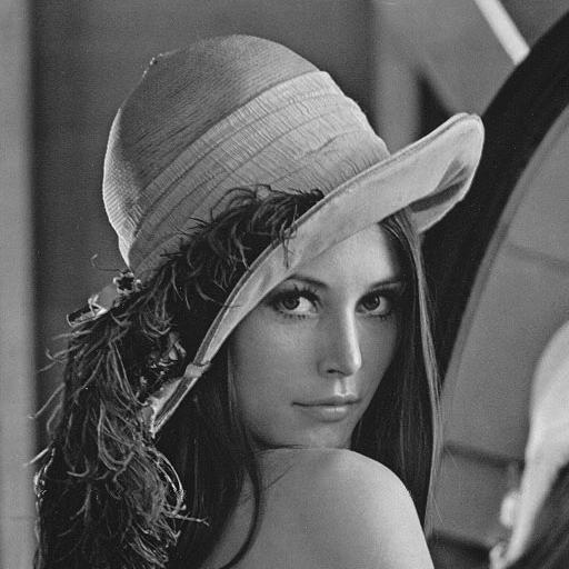
For this example we use an external package image
require 'image'
require 'nn'
lena = image.rgb2y(image.lena())
ker = torch.ones(11)
m=nn.SpatialSubtractiveNormalization(1,ker)
processed = m:forward(lena)
w1=image.display(lena)
w2=image.display(processed)

Volumetric Modules
Excluding and optional batch dimension, volumetric layers expect a 4D Tensor as input. The
first dimension is the number of features (e.g. frameSize), the second is sequential (e.g. time) and the
last two dimenstions are spatial (e.g. height x width). These are commonly used for processing videos (sequences of images).
VolumetricConvolution
module = nn.VolumetricConvolution(nInputPlane, nOutputPlane, kT, kW, kH [, dT, dW, dH])
Applies a 3D convolution over an input image composed of several input planes. The input tensor in
forward(input) is expected to be a 4D tensor (nInputPlane x time x height x width).
The parameters are the following:
* nInputPlane: The number of expected input planes in the image given into forward().
* nOutputPlane: The number of output planes the convolution layer will produce.
* kT: The kernel size of the convolution in time
* kW: The kernel width of the convolution
* kH: The kernel height of the convolution
* dT: The step of the convolution in the time dimension. Default is 1.
* dW: The step of the convolution in the width dimension. Default is 1.
* dH: The step of the convolution in the height dimension. Default is 1.
Note that depending of the size of your kernel, several (of the last) columns or rows of the input image might be lost. It is up to the user to add proper padding in images.
If the input image is a 4D tensor nInputPlane x time x height x width, the output image size
will be nOutputPlane x otime x owidth x oheight where
otime   = (time  - kT) / dT + 1
owidth  = (width  - kW) / dW + 1
oheight = (height - kH) / dH + 1 .
The parameters of the convolution can be found in self.weight (Tensor of
size nOutputPlane x nInputPlane x kT x kH x kW) and self.bias (Tensor of
size nOutputPlane). The corresponding gradients can be found in
self.gradWeight and self.gradBias.
VolumetricMaxPooling
module = nn.VolumetricMaxPooling(kT, kW, kH [, dT, dW, dH])
Applies 3D max-pooling operation in kTxkWxkH regions by step size
dTxdWxdH steps. The number of output features is equal to the number of
input planes.