Transfer Function Layers

Transfer functions are normally used to introduce a non-linearity after a parameterized layer like Linear and SpatialConvolution. Non-linearities allows for dividing the problem space into more complex regions than what a simple logistic regressor would permit.

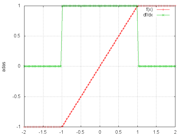
HardTanh

f = nn.HardTanh([min_value, max_value[, inplace]])

Applies the HardTanh function element-wise to the input Tensor, thus outputting a Tensor of the same dimension.

HardTanh is defined as:

       ⎧  1, if x >  1
f(x) = ⎨ -1, if x < -1
       ⎩  x, otherwise

The range of the linear region [-1 1] can be adjusted by specifying arguments in declaration, for example nn.HardTanh(min_value, max_value). Otherwise, [min_value max_value] is set to [-1 1] by default. In-place operation defined by third argument boolean.

ii = torch.linspace(-2, 2)
m = nn.HardTanh()
oo = m:forward(ii)
go = torch.ones(100)
gi = m:backward(ii, go)
gnuplot.plot({'f(x)', ii, oo, '+-'}, {'df/dx', ii, gi, '+-'})
gnuplot.grid(true)

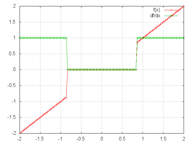
HardShrink

f = nn.HardShrink([lambda])

Applies the hard shrinkage function element-wise to the input Tensor. lambda is set to 0.5 by default.

HardShrinkage operator is defined as:

       ⎧ x, if x >  lambda
f(x) = ⎨ x, if x < -lambda
       ⎩ 0, otherwise

ii = torch.linspace(-2, 2)
m = nn.HardShrink(0.85)
oo = m:forward(ii)
go = torch.ones(100)
gi = m:backward(ii, go)
gnuplot.plot({'f(x)', ii, oo, '+-'}, {'df/dx', ii, gi, '+-'})
gnuplot.grid(true)

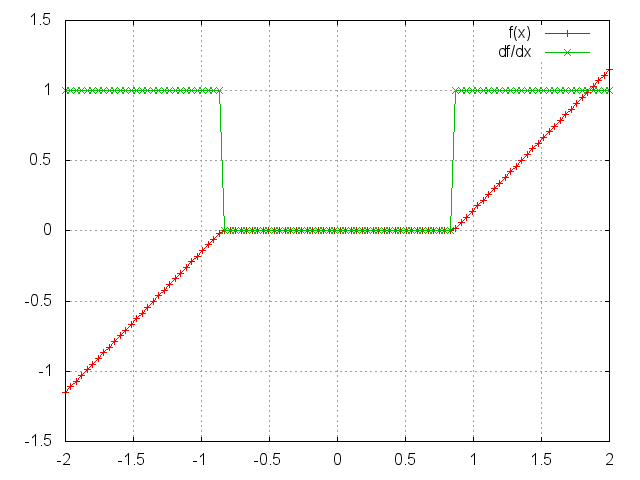
SoftShrink

f = nn.SoftShrink([lambda])

Applies the soft shrinkage function element-wise to the input Tensor. lambda is set to 0.5 by default.

SoftShrinkage operator is defined as:

       ⎧ x - lambda, if x >  lambda
f(x) = ⎨ x + lambda, if x < -lambda
       ⎩ 0, otherwise

ii = torch.linspace(-2, 2)
m = nn.SoftShrink(0.85)
oo = m:forward(ii)
go = torch.ones(100)
gi = m:backward(ii, go)
gnuplot.plot({'f(x)', ii, oo, '+-'}, {'df/dx', ii, gi, '+-'})
gnuplot.grid(true)

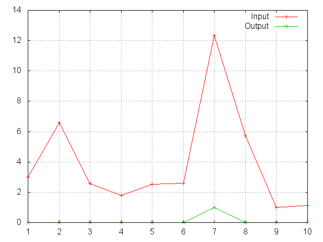
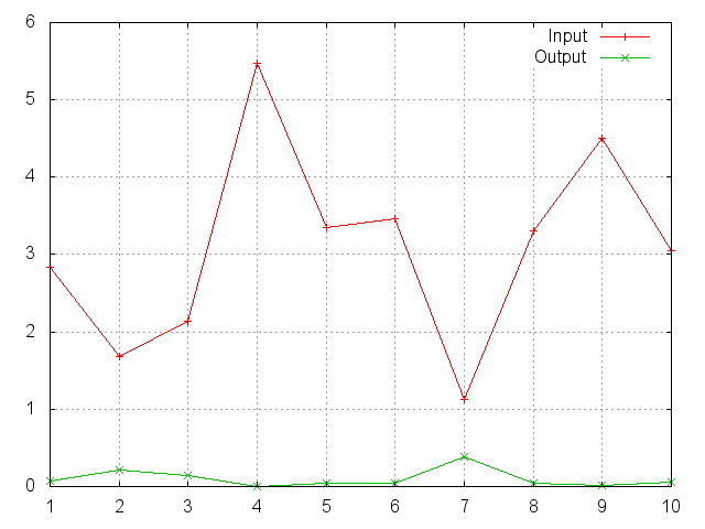
SoftMax

f = nn.SoftMax()

Applies the SoftMax function to an n-dimensional input Tensor, rescaling them so that the elements of the n-dimensional output Tensor lie in the range (0, 1) and sum to 1.

Softmax is defined as:

f_i(x) = exp(x_i - shift) / sum_j exp(x_j - shift)

where shift = max_i(x_i).

ii = torch.exp(torch.abs(torch.randn(10)))
m = nn.SoftMax()
oo = m:forward(ii)
gnuplot.plot({'Input', ii, '+-'}, {'Output', oo, '+-'})
gnuplot.grid(true)

Note that this module doesn't work directly with ClassNLLCriterion, which expects the nn.Log to be computed between the SoftMax and itself. Use LogSoftMax instead (it's faster).

SoftMin

f = nn.SoftMin()

Applies the SoftMin function to an n-dimensional input Tensor, rescaling them so that the elements of the n-dimensional output Tensor lie in the range (0,1) and sum to 1.

Softmin is defined as:

f_i(x) = exp(-x_i - shift) / sum_j exp(-x_j - shift)

where shift = max_i(-x_i).

ii = torch.exp(torch.abs(torch.randn(10)))
m = nn.SoftMin()
oo = m:forward(ii)
gnuplot.plot({'Input', ii, '+-'}, {'Output', oo, '+-'})
gnuplot.grid(true)

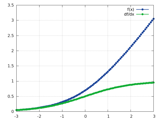
SoftPlus

f = nn.SoftPlus()

Applies the SoftPlus function to an n-dimensioanl input Tensor. SoftPlus is a smooth approximation to the ReLU function and can be used to constrain the output of a machine to always be positive. For numerical stability the implementation reverts to the linear function for inputs above a certain value (20 by default).

SoftPlus is defined as:

f_i(x) = 1/beta * log(1 + exp(beta * x_i))

ii = torch.linspace(-3, 3)
m = nn.SoftPlus()
oo = m:forward(ii)
go = torch.ones(100)
gi = m:backward(ii, go)
gnuplot.plot({'f(x)', ii, oo, '+-'}, {'df/dx', ii, gi, '+-'})
gnuplot.grid(true)

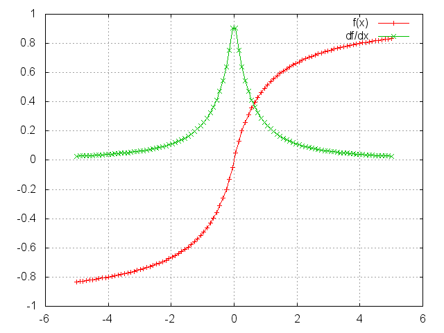
SoftSign

f = nn.SoftSign()

Applies the SoftSign function to an n-dimensioanl input Tensor.

SoftSign is defined as:

f_i(x) = x_i / (1+|x_i|)

ii = torch.linspace(-5, 5)
m = nn.SoftSign()
oo = m:forward(ii)
go = torch.ones(100)
gi = m:backward(ii, go)
gnuplot.plot({'f (x)', ii, oo, '+-'}, {'df/dx', ii, gi, '+-'})
gnuplot.grid(true)

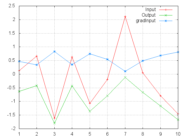
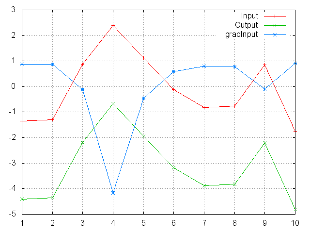
LogSigmoid

f = nn.LogSigmoid()

Applies the LogSigmoid function to an n-dimensional input Tensor.

LogSigmoid is defined as:

f_i(x) = log(1 / (1 + exp(-x_i)))

ii = torch.randn(10)
m = nn.LogSigmoid()
oo = m:forward(ii)
go = torch.ones(10)
gi = m:backward(ii, go)
gnuplot.plot({'Input', ii, '+-'}, {'Output', oo, '+-'}, {'gradInput', gi, '+-'})
gnuplot.grid(true)

LogSoftMax

f = nn.LogSoftMax()

Applies the LogSoftMax function to an n-dimensional input Tensor.

LogSoftmax is defined as:

f_i(x) = log(1 / a exp(x_i))

where a = sum_j[exp(x_j)].

ii = torch.randn(10)
m = nn.LogSoftMax()
oo = m:forward(ii)
go = torch.ones(10)
gi = m:backward(ii, go)
gnuplot.plot({'Input', ii, '+-'}, {'Output', oo, '+-'}, {'gradInput', gi, '+-'})
gnuplot.grid(true)

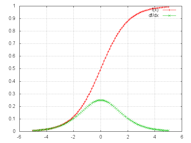
Sigmoid

f = nn.Sigmoid()

Applies the Sigmoid function element-wise to the input Tensor, thus outputting a Tensor of the same dimension.

Sigmoid is defined as:

f(x) = 1 / (1 + exp(-x))

ii = torch.linspace(-5, 5)
m = nn.Sigmoid()
oo = m:forward(ii)
go = torch.ones(100)
gi = m:backward(ii, go)
gnuplot.plot({'f(x)', ii, oo, '+-'}, {'df/dx', ii, gi, '+-'})
gnuplot.grid(true)

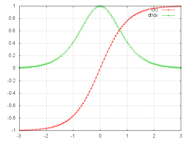
Tanh

f = nn.Tanh()

Applies the Tanh function element-wise to the input Tensor, thus outputting a Tensor of the same dimension.

Tanh is defined as:

f(x) = (exp(x) - exp(-x)) / (exp(x) + exp(-x))

ii = torch.linspace(-3, 3)
m = nn.Tanh()
oo = m:forward(ii)
go = torch.ones(100)
gi = m:backward(ii, go)
gnuplot.plot({'f(x)', ii, oo, '+-'}, {'df/dx', ii, gi, '+-'})
gnuplot.grid(true)

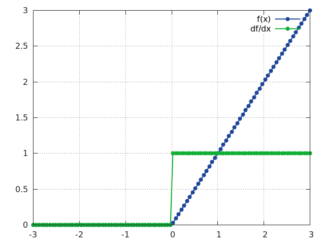
ReLU

f = nn.ReLU([inplace])

Applies the rectified linear unit (ReLU) function element-wise to the input Tensor, thus outputting a Tensor of the same dimension.

ReLU is defined as:

f(x) = max(0, x)

Can optionally do its operation in-place without using extra state memory:

f = nn.ReLU(true) -- true = in-place, false = keeping separate state.

ii = torch.linspace(-3, 3)
m = nn.ReLU()
oo = m:forward(ii)
go = torch.ones(100)
gi = m:backward(ii, go)
gnuplot.plot({'f(x)', ii, oo, '+-'}, {'df/dx', ii, gi, '+-'})
gnuplot.grid(true)

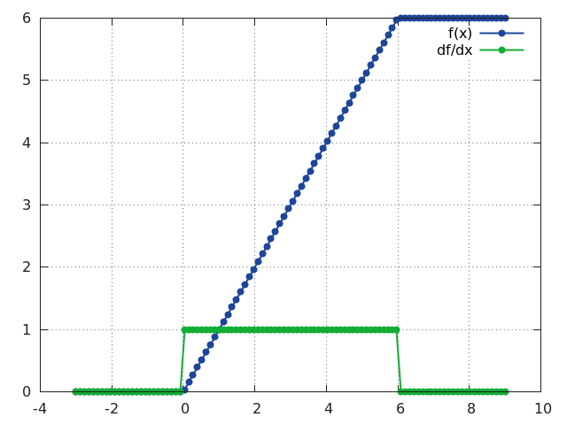
ReLU6

f = nn.ReLU6([inplace])

Same as ReLU except that the rectifying function f(x) saturates at x = 6. This layer is useful for training networks that do not loose precision (due to FP saturation) when implemented as FP16.

ReLU6 is defined as:

f(x) = min(max(0, x), 6)

Can optionally do its operation in-place without using extra state memory:

f = nn.ReLU6(true) -- true = in-place, false = keeping separate state.

ii = torch.linspace(-3, 9)
m = nn.ReLU6()
oo = m:forward(ii)
go = torch.ones(100)
gi = m:backward(ii, go)
gnuplot.plot({'f(x)', ii, oo, '+-'}, {'df/dx', ii, gi, '+-'})
gnuplot.grid(true)

PReLU

f = nn.PReLU()

Applies parametric ReLU, which parameter varies the slope of the negative part:

PReLU is defined as:

f(x) = max(0, x) + a * min(0, x)

When called without a number on input as nn.PReLU() uses shared version, meaning has only one parameter. Otherwise if called nn.PReLU(nOutputPlane) has nOutputPlane parameters, one for each input map. The output dimension is always equal to input dimension. Note that weight decay should not be used on it. For reference see Delving Deep into Rectifiers.

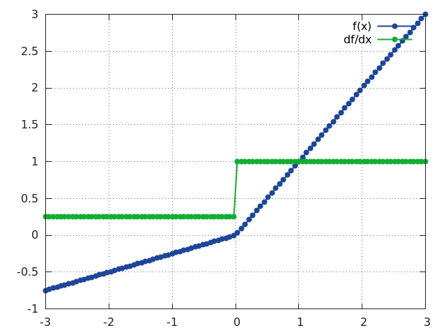
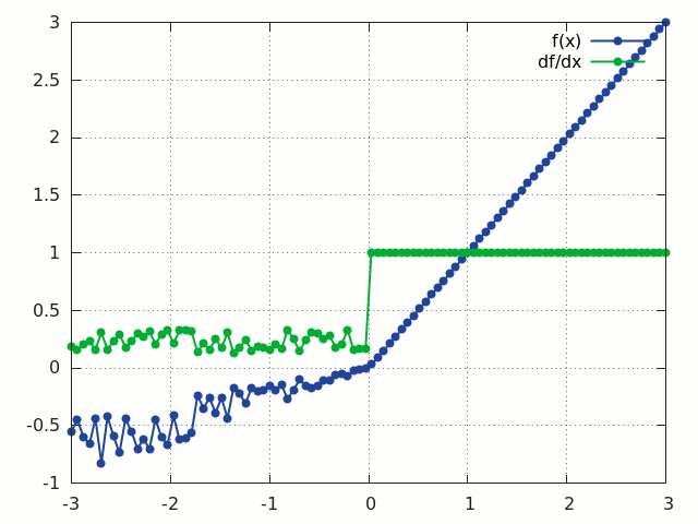
RReLU

f = nn.RReLU([l, u[, inplace]])

Applies the randomized leaky rectified linear unit (RReLU) element-wise to the input Tensor, thus outputting a Tensor of the same dimension. Informally the RReLU is also known as 'insanity' layer.

RReLU is defined as:

f(x) = max(0,x) + a * min(0, x)

where a ~ U(l, u).

In training mode negative inputs are multiplied by a factor a drawn from a uniform random distribution U(l, u). In evaluation mode a RReLU behaves like a LeakyReLU with a constant mean factor a = (l + u) / 2. By default, l = 1/8 and u = 1/3. If l == u a RReLU effectively becomes a LeakyReLU. Regardless of operating in in-place mode a RReLU will internally allocate an input-sized noise tensor to store random factors for negative inputs. The backward() operation assumes that forward() has been called before.

For reference see Empirical Evaluation of Rectified Activations in Convolutional Network.

ii = torch.linspace(-3, 3)
m = nn.RReLU()
oo = m:forward(ii):clone()
gi = m:backward(ii, torch.ones(100))
gnuplot.plot({'f(x)', ii, oo, '+-'}, {'df/dx', ii, gi, '+-'})
gnuplot.grid(true)

CReLU

f = nn.CReLU(nInputDims, [inplace])

Applies the Concatenated Rectified Linear Unit (CReLU) function to the input Tensor, outputting a Tensor with twice as many channels. The parameter nInputDim is the number of non-batched dimensions, larger than that value will be considered batches. CReLU is defined as:

f(x) = concat(max(0, x), max(0, -x))

i.e. CReLU applies ReLU to the input, x, and the negated input, -x, and concatenates the output along the 1st non-batched dimension.

crelu = nn.CReLU(3)
input = torch.Tensor(2, 3, 20, 20):uniform(-1, 1)
output = crelu:forward(input)
output:size()
2
6
20
20
[torch.LongStorage of size 4]

input = torch.Tensor(3, 20, 20):uniform(-1, 1)
output = crelu:forward(input)
output:size()
6
20
20
[torch.LongStorage of size 3]

For reference see Understanding and Improving Convolutional Neural Networks via Concatenated Rectified Linear Units.

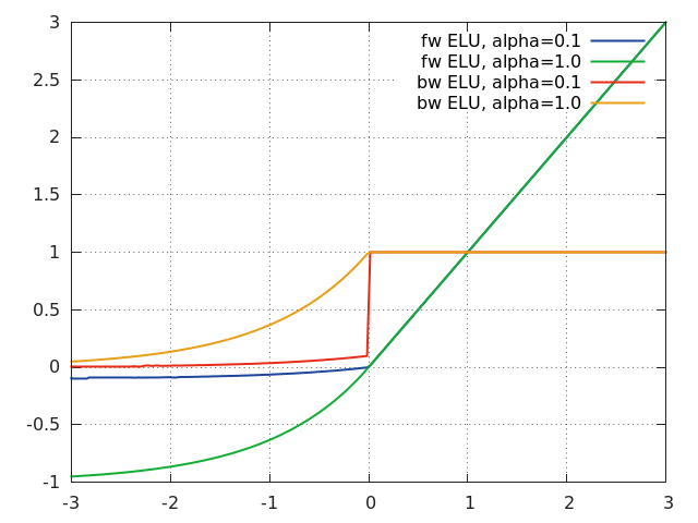
ELU

f = nn.ELU([alpha[, inplace]])

Applies exponential linear unit (ELU), which parameter a varies the convergence value of the exponential function below zero:

ELU is defined as:

f(x) = max(0, x) + min(0, alpha * (exp(x) - 1))

The output dimension is always equal to input dimension.

For reference see Fast and Accurate Deep Network Learning by Exponential Linear Units (ELUs).

xs = torch.linspace(-3, 3, 200)
go = torch.ones(xs:size(1))
function f(a) return nn.ELU(a):forward(xs) end
function df(a) local m = nn.ELU(a) m:forward(xs) return m:backward(xs, go) end

gnuplot.plot({'fw ELU, alpha = 0.1', xs,  f(0.1), '-'},
             {'fw ELU, alpha = 1.0', xs,  f(1.0), '-'},
             {'bw ELU, alpha = 0.1', xs, df(0.1), '-'},
             {'bw ELU, alpha = 1.0', xs, df(1.0), '-'})
gnuplot.grid(true)

LeakyReLU

f = nn.LeakyReLU([negval[, inplace]])

Applies LeakyReLU, which parameter negval sets the slope of the negative part:

LeakyReLU is defined as:

f(x) = max(0, x) + negval * min(0, x)

Can optionally do its operation in-place without using extra state memory:

f = nn.LeakyReLU(negval, true) -- true = in-place, false = keeping separate state.

GatedLinearUnit

Applies a Gated Linear unit activation function, which halves the input dimension as follows:

GatedLinearUnit is defined as f([x1, x2]) = x1 * sigmoid(x2)

where x1 is the first half of the input vector and x2 is the second half. The multiplication is component-wise, and the input vector must have an even number of elements.

The GatedLinearUnit optionally takes a dim parameter, which is the dimension of the input tensor to operate over. It defaults to the last dimension.

SpatialSoftMax

f = nn.SpatialSoftMax()

Applies SoftMax over features to each spatial location (height x width of planes). The module accepts 1D (vector), 2D (batch of vectors), 3D (vectors in space) or 4D (batch of vectors in space) Tensor as input. Functionally it is equivalent to SoftMax when 1D or 2D input is used. The output dimension is always the same as input dimension.

ii = torch.randn(4, 8, 16, 16)  -- batchSize x features x height x width
m = nn.SpatialSoftMax()
oo = m:forward(ii)

SpatialLogSoftMax

Applies LogSoftMax over features to each spatial location (height x width of planes). The module accepts 1D (vector), 2D (batch of vectors), 3D (vectors in space) or 4D (batch of vectors in space) tensor as input. Functionally it is equivalent to LogSoftMax when 1D or 2D input is used. The output dimension is always the same as input dimension.

ii=torch.randn(4,8,16,16)  -- batchSize x features x height x width
m=nn.SpatialLogSoftMax()
oo = m:forward(ii)

AddConstant

f = nn.AddConstant(k[, inplace])

Adds a (non-learnable) scalar constant. This module is sometimes useful for debugging purposes. Its transfer function is:

f(x) = x + k

where k is a scalar.

Can optionally do its operation in-place without using extra state memory:

f = nn.AddConstant(k, true) -- true = in-place, false = keeping separate state.

In-place mode restores the original input value after the backward pass, allowing its use after other in-place modules, like MulConstant.

MulConstant

f = nn.MulConstant(k[, inplace])

Multiplies input Tensor by a (non-learnable) scalar constant. This module is sometimes useful for debugging purposes. Its transfer function is:

f(x) = k * x

where k is a scalar.

Can optionally do its operation in-place without using extra state memory:

m = nn.MulConstant(k, true) -- true = in-place, false = keeping separate state.

In-place mode restores the original input value after the backward pass, allowing its use after other in-place modules, like AddConstant.