Simple layers
Simple Modules are used for various tasks like adapting Tensor methods and providing affine transformations :
- Parameterized Modules :
- Linear : a linear transformation ;
- SparseLinear : a linear transformation with sparse inputs ;
- Add : adds a bias term to the incoming data ;
- Mul : multiply a single scalar factor to the incoming data ;
- CMul : a component-wise multiplication to the incoming data ;
- CDiv : a component-wise division to the incoming data ;
- Euclidean : the euclidean distance of the input to
kmean centers ; - WeightedEuclidean : similar to Euclidean, but additionally learns a diagonal covariance matrix ;
- Modules that adapt basic Tensor methods :
- Modules that adapt mathematical Tensor methods :
- Max : a max operation over a given dimension ;
- Min : a min operation over a given dimension ;
- Mean : a mean operation over a given dimension ;
- Sum : a sum operation over a given dimension ;
- Exp : an element-wise exp operation ;
- Abs : an element-wise abs operation ;
- Power : an element-wise pow operation ;
- Square : an element-wise square operation ;
- Sqrt : an element-wise sqrt operation ;
- MM : matrix-matrix multiplication (also supports batches of matrices) ;
- Miscellaneous Modules :
- Identity : forward input as-is to output (useful with ParallelTable);
- Dropout : masks parts of the
inputusing binary samples from a bernoulli distribution ;
Linear
module = Linear(inputDimension,outputDimension)
Applies a linear transformation to the incoming data, i.e. //y=
Ax+b//. The input tensor given in forward(input) must be
either a vector (1D tensor) or matrix (2D tensor). If the input is a
matrix, then each row is assumed to be an input sample of given batch.
You can create a layer in the following way:
module= nn.Linear(10,5) -- 10 inputs, 5 outputs
Usually this would be added to a network of some kind, e.g.:
 mlp = nn.Sequential();
 mlp:add(module)
The weights and biases (A and b) can be viewed with:
 print(module.weight)
 print(module.bias)
The gradients for these weights can be seen with:
 print(module.gradWeight)
 print(module.gradBias)
As usual with nn modules,
applying the linear transformation is performed with:
 x=torch.Tensor(10) -- 10 inputs
 y=module:forward(x)
SparseLinear
module = SparseLinear(inputDimension,outputDimension)
Applies a linear transformation to the incoming sparse data, i.e.
y= Ax+b. The input tensor given in forward(input) must
be a sparse vector represented as 2D tensor of the form
torch.Tensor(N, 2) where the pairs represent indices and values.
The SparseLinear layer is useful when the number of input
dimensions is very large and the input data is sparse.
You can create a sparse linear layer in the following way:
module= nn.SparseLinear(10000,2) -- 10000 inputs, 2 outputs
The sparse linear module may be used as part of a larger network, and apart from the form of the input, SparseLinear operates in exactly the same way as the Linear layer.
A sparse input vector may be created as so..
 x=torch.Tensor({{1, 0.1},{2, 0.3},{10, 0.3},{31, 0.2}})

 print(x)

  1.0000   0.1000
  2.0000   0.3000
 10.0000   0.3000
 31.0000   0.2000
[torch.Tensor of dimension 4x2]
The first column contains indices, the second column contains values in a a vector where all other elements are zeros. The indices should not exceed the stated dimensions of the input to the layer (10000 in the example).
Dropout
module = nn.Dropout(p)
During training, Dropout masks parts of the input using binary samples from
a bernoulli distribution.
Each input element has a probability of p of being dropped, i.e having its
commensurate output element be zero. This has proven an effective technique for
regularization and preventing the co-adaptation of neurons
(see Hinton et al. 2012).
Furthermore, the ouputs are scaled by a factor of 1/(1-p) during training. This allows the
input to be simply forwarded as-is during evaluation.
In this example, we demonstrate how the call to forward samples
different outputs to dropout (the zeros) given the same input:
module = nn.Dropout()

> x=torch.Tensor{{1,2,3,4},{5,6,7,8}}

> =module:forward(x)
  2   0   0   8
 10   0  14   0
[torch.DoubleTensor of dimension 2x4]

> =module:forward(x)
  0   0   6   0
 10   0   0   0
[torch.DoubleTensor of dimension 2x4]
Backward drops out the gradients at the same location:
> =module:forward(x)
  0   4   0   0
 10  12   0  16
[torch.DoubleTensor of dimension 2x4]

> =module:backward(x,x:clone():fill(1))
 0  2  0  0
 2  2  0  2
[torch.DoubleTensor of dimension 2x4]
In both cases the gradOutput and input are scaled by 1/(1-p), which in this case is 2.
During evaluation, Dropout does nothing more than
forward the input such that all elements of the input are considered.
> module:evaluate()

> module:forward(x)
 1  2  3  4
 5  6  7  8
[torch.DoubleTensor of dimension 2x4]
We can return to training our model by first calling Module:training():
> module:training()

> return module:forward(x)
  2   4   6   0
  0   0   0  16
[torch.DoubleTensor of dimension 2x4]
When used, Dropout should normally be applied to the input of parameterized
Modules like Linear
or SpatialConvolution.
A p of 0.5 (the default) is usually okay for hidden layers.
Dropout can sometimes be used successfully on the dataset inputs with a p around 0.2.
It sometimes works best following Transfer Modules
like ReLU. All this depends a great deal on the dataset so its up
to the user to try different combinations.
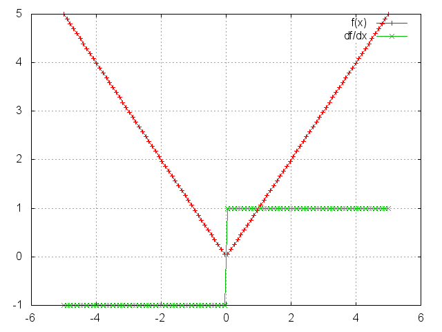
Abs
module = Abs()
output = abs(input).
m=nn.Abs()
ii=torch.linspace(-5,5)
oo=m:forward(ii)
go=torch.ones(100)
gi=m:backward(ii,go)
gnuplot.plot({'f(x)',ii,oo,'+-'},{'df/dx',ii,gi,'+-'})
gnuplot.grid(true)
Add
module = Add(inputDimension,scalar)
Applies a bias term to the incoming data, i.e. y_i= x_i + b_i, or if _scalar=true then uses a single bias term, _y_i= x_i + b.
Example:
y=torch.Tensor(5);
mlp=nn.Sequential()
mlp:add(nn.Add(5))

function gradUpdate(mlp, x, y, criterion, learningRate)
  local pred = mlp:forward(x)
  local err = criterion:forward(pred, y)
  local gradCriterion = criterion:backward(pred, y)
  mlp:zeroGradParameters()
  mlp:backward(x, gradCriterion)
  mlp:updateParameters(learningRate)
  return err
end

for i=1,10000 do
 x=torch.rand(5)
 y:copy(x);
 for i=1,5 do y[i]=y[i]+i; end
 err=gradUpdate(mlp,x,y,nn.MSECriterion(),0.01)
end
print(mlp:get(1).bias)
gives the output:
 1.0000
 2.0000
 3.0000
 4.0000
 5.0000
[torch.Tensor of dimension 5]
i.e. the network successfully learns the input x has been shifted to produce the output y.
Mul
module = Mul()
Applies a single scaling factor to the incoming data, i.e. y= w x, where w is a scalar.
Example:
y=torch.Tensor(5);
mlp=nn.Sequential()
mlp:add(nn.Mul())

function gradUpdate(mlp, x, y, criterion, learningRate)
  local pred = mlp:forward(x)
  local err = criterion:forward(pred,y)
  local gradCriterion = criterion:backward(pred,y);
  mlp:zeroGradParameters();
  mlp:backward(x, gradCriterion);
  mlp:updateParameters(learningRate);
  return err
end


for i=1,10000 do
 x=torch.rand(5)
 y:copy(x); y:mul(math.pi);
 err=gradUpdate(mlp,x,y,nn.MSECriterion(),0.01)
end
print(mlp:get(1).weight)
gives the output:
 3.1416
[torch.Tensor of dimension 1]
i.e. the network successfully learns the input x has been scaled by
pi.
CMul
module = CMul(size)
Applies a component-wise multiplication to the incoming data, i.e.
y_i = w_i * x_i. Argument size can be one or many numbers (sizes)
or a torch.LongStorage. For example, nn.CMul(3,4,5) is equivalent to
nn.CMul(torch.LongStorage{3,4,5}).
Example:
mlp=nn.Sequential()
mlp:add(nn.CMul(5))

y=torch.Tensor(5);
sc=torch.Tensor(5); for i=1,5 do sc[i]=i; end -- scale input with this

function gradUpdate(mlp,x,y,criterion,learningRate)
  local pred = mlp:forward(x)
  local err = criterion:forward(pred,y)
  local gradCriterion = criterion:backward(pred,y);
  mlp:zeroGradParameters();
  mlp:backward(x, gradCriterion);
  mlp:updateParameters(learningRate);
  return err
end

for i=1,10000 do
 x=torch.rand(5)
 y:copy(x); y:cmul(sc);
 err=gradUpdate(mlp,x,y,nn.MSECriterion(),0.01)
end
print(mlp:get(1).weight)
gives the output:
 1.0000
 2.0000
 3.0000
 4.0000
 5.0000
[torch.Tensor of dimension 5]
i.e. the network successfully learns the input x has been scaled by those scaling factors to produce the output y.
Max
module = Max(dimension)
Applies a max operation over dimension dimension.
Hence, if an nxpxq Tensor was given as input, and dimension = 2
then an nxq matrix would be output.
Min
module = Min(dimension)
Applies a min operation over dimension dimension.
Hence, if an nxpxq Tensor was given as input, and dimension = 2
then an nxq matrix would be output.
Mean
module = Mean(dimension)
Applies a mean operation over dimension dimension.
Hence, if an nxpxq Tensor was given as input, and dimension = 2
then an nxq matrix would be output.
Sum
module = Sum(dimension)
Applies a sum operation over dimension dimension.
Hence, if an nxpxq Tensor was given as input, and dimension = 2
then an nxq matrix would be output.
Euclidean
module = Euclidean(inputSize,outputSize)
Outputs the Euclidean distance of the input to outputSize centers,
i.e. this layer has the weights w_j, for j = 1,..,outputSize, where
w_j are vectors of dimension inputSize.
The distance y_j between center j and input x is formulated as
y_j = || w_j - x ||.
WeightedEuclidean
module = WeightedEuclidean(inputSize,outputSize)
This module is similar to Euclidean, but additionally learns a separate diagonal covariance matrix across the features of the input space for each center.
In other words, for each of the outputSize centers w_j, there is
a diagonal covariance matrices c_j, for j = 1,..,outputSize,
where c_j are stored as vectors of size inputSize.
The distance y_j between center j and input x is formulated as
y_j = || c_j * (w_j - x) ||.
Identity
module = Identity()
Creates a module that returns whatever is input to it as output. This is useful when combined with the module ParallelTable in case you do not wish to do anything to one of the input Tensors. Example:
mlp=nn.Identity()
print(mlp:forward(torch.ones(5,2)))
gives the output:
 1  1
 1  1
 1  1
 1  1
 1  1
[torch.Tensor of dimension 5x2]
Here is a more useful example, where one can implement a network which also computes a Criterion using this module:
pred_mlp=nn.Sequential(); -- A network that makes predictions given x.
pred_mlp:add(nn.Linear(5,4))
pred_mlp:add(nn.Linear(4,3))

xy_mlp=nn.ParallelTable();-- A network for predictions and for keeping the
xy_mlp:add(pred_mlp)      -- true label for comparison with a criterion
xy_mlp:add(nn.Identity()) -- by forwarding both x and y through the network.

mlp=nn.Sequential();     -- The main network that takes both x and y.
mlp:add(xy_mlp)      -- It feeds x and y to parallel networks;
cr=nn.MSECriterion();
cr_wrap=nn.CriterionTable(cr)
mlp:add(cr_wrap)         -- and then applies the criterion.

for i=1,100 do       -- Do a few training iterations
  x=torch.ones(5);          -- Make input features.
  y=torch.Tensor(3);
  y:copy(x:narrow(1,1,3)) -- Make output label.
  err=mlp:forward{x,y}    -- Forward both input and output.
  print(err)         -- Print error from criterion.

  mlp:zeroGradParameters();  -- Do backprop...
  mlp:backward({x, y} );
  mlp:updateParameters(0.05);
end
Copy
module = Copy(inputType,outputType,[forceCopy,dontCast])
This layer copies the input to output with type casting from input
type from inputType to outputType. Unless forceCopy is true, when
the first two arguments are the same, the input isn't copied, only transfered
as the output. The default forceCopy is false.
When dontCast is true, a call to nn.Copy:type(type) will not cast
the module's output and gradInput Tensors to the new type. The default
is false.
Narrow
module = Narrow(dimension, offset, length)
Narrow is application of narrow operation in a module.
Replicate
module = Replicate(nFeature)
This class creates an output where the input is replicated
nFeature times along its first dimension. There is no memory
allocation or memory copy in this module. It sets the
stride along the first
dimension to zero.
torch> x=torch.linspace(1,5,5)
torch> =x
 1
 2
 3
 4
 5
[torch.DoubleTensor of dimension 5]

torch> m=nn.Replicate(3)
torch> o=m:forward(x)
torch> =o
 1  2  3  4  5
 1  2  3  4  5
 1  2  3  4  5
[torch.DoubleTensor of dimension 3x5]

torch> x:fill(13)
torch> =x
 13
 13
 13
 13
 13
[torch.DoubleTensor of dimension 5]

torch> =o
 13  13  13  13  13
 13  13  13  13  13
 13  13  13  13  13
[torch.DoubleTensor of dimension 3x5]
Reshape
module = Reshape(dimension1, dimension2, ... [, batchMode])
Reshapes an nxpxqx.. Tensor into a dimension1xdimension2x... Tensor,
taking the elements column-wise.
The optional last argument batchMode,
when true forces the first dimension of the input to be considered
the batch dimension, and thus keep its size fixed. This is necessary when
dealing with batch sizes of one. When false, it forces the
entire input (including the first dimension) to be reshaped to the
input size. Default batchMode=nil, which means that the module
considers inputs with more elements than the produce of provided sizes,
i.e. dimension1xdimension2x..., to be batches.
Example:
> x=torch.Tensor(4,4)
> for i=1,4 do
>  for j=1,4 do
>   x[i][j]=(i-1)*4+j;
>  end
> end
> print(x)

  1   2   3   4
  5   6   7   8
  9  10  11  12
 13  14  15  16
[torch.Tensor of dimension 4x4]

> print(nn.Reshape(2,8):forward(x))

  1   9   2  10   3  11   4  12
  5  13   6  14   7  15   8  16
[torch.Tensor of dimension 2x8]

> print(nn.Reshape(8,2):forward(x))

  1   3
  5   7
  9  11
 13  15
  2   4
  6   8
 10  12
 14  16
[torch.Tensor of dimension 8x2]

> print(nn.Reshape(16):forward(x))

  1
  5
  9
 13
  2
  6
 10
 14
  3
  7
 11
 15
  4
  8
 12
 16
[torch.Tensor of dimension 16]
View
module = View(sizes)
This module creates a new view of the input tensor using the sizes passed to
the constructor. The parameter sizes can either be a LongStorage or numbers.
The method setNumInputDims() allows to specify the expected number of dimensions
of the inputs of the modules. This makes it possible to use minibatch inputs when
using a size -1 for one of the dimensions.
Example 1:
> x=torch.Tensor(4,4)
> for i=1,4 do
>  for j=1,4 do
>   x[i][j]=(i-1)*4+j;
>  end
> end
> print(x)

  1   2   3   4
  5   6   7   8
  9  10  11  12
 13  14  15  16
[torch.Tensor of dimension 4x4]

> print(nn.View(2,8):forward(x))

  1   2   3   4   5   6   7   8
  9  10  11  12  13  14  15  16
[torch.DoubleTensor of dimension 2x8]

> print(nn.View(torch.LongStorage{8,2}):forward(x))

  1   2
  3   4
  5   6
  7   8
  9  10
 11  12
 13  14
 15  16
[torch.DoubleTensor of dimension 8x2]

> print(nn.View(16):forward(x))

  1
  2
  3
  4
  5
  6
  7
  8
  9
 10
 11
 12
 13
 14
 15
 16
[torch.DoubleTensor of dimension 16]
Example 2:
> input = torch.Tensor(2,3)
> minibatch = torch.Tensor(5,2,3)
> m = nn.View(-1):setNumInputDims(2)
> print(#m:forward(input))

 6
[torch.LongStorage of size 2]

> print(#m:forward(minibatch))

 5
 6
[torch.LongStorage of size 2]
Select
Selects a dimension and index of a nxpxqx.. Tensor.
Example:
mlp=nn.Sequential();
mlp:add(nn.Select(1,3))

x=torch.randn(10,5)
print(x)
print(mlp:forward(x))
gives the output:
 0.9720 -0.0836  0.0831 -0.2059 -0.0871
 0.8750 -2.0432 -0.1295 -2.3932  0.8168
 0.0369  1.1633  0.6483  1.2862  0.6596
 0.1667 -0.5704 -0.7303  0.3697 -2.2941
 0.4794  2.0636  0.3502  0.3560 -0.5500
-0.1898 -1.1547  0.1145 -1.1399  0.1711
-1.5130  1.4445  0.2356 -0.5393 -0.6222
-0.6587  0.4314  1.1916 -1.4509  1.9400
 0.2733  1.0911  0.7667  0.4002  0.1646
 0.5804 -0.5333  1.1621  1.5683 -0.1978
[torch.Tensor of dimension 10x5]

 0.0369
 1.1633
 0.6483
 1.2862
 0.6596
[torch.Tensor of dimension 5]
This can be used in conjunction with Concat to emulate the behavior of Parallel, or to select various parts of an input Tensor to perform operations on. Here is a fairly complicated example:
mlp=nn.Sequential();
c=nn.Concat(2)
for i=1,10 do
 local t=nn.Sequential()
 t:add(nn.Select(1,i))
 t:add(nn.Linear(3,2))
 t:add(nn.Reshape(2,1))
 c:add(t)
end
mlp:add(c)

pred=mlp:forward(torch.randn(10,3))
print(pred)

for i=1,10000 do     -- Train for a few iterations
 x=torch.randn(10,3);
 y=torch.ones(2,10);
 pred=mlp:forward(x)

 criterion= nn.MSECriterion()
 err=criterion:forward(pred,y)
 gradCriterion = criterion:backward(pred,y);
 mlp:zeroGradParameters();
 mlp:backward(x, gradCriterion);
 mlp:updateParameters(0.01);
 print(err)
end
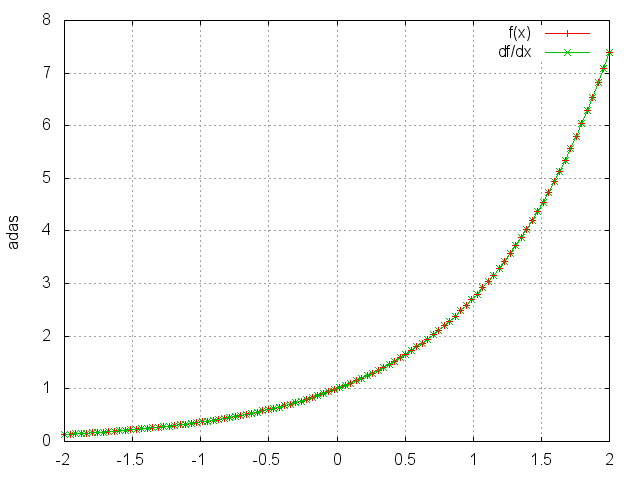
Exp
Applies the exp function element-wise to the input Tensor,
thus outputting a Tensor of the same dimension.
ii=torch.linspace(-2,2)
m=nn.Exp()
oo=m:forward(ii)
go=torch.ones(100)
gi=m:backward(ii,go)
gnuplot.plot({'f(x)',ii,oo,'+-'},{'df/dx',ii,gi,'+-'})
gnuplot.grid(true)
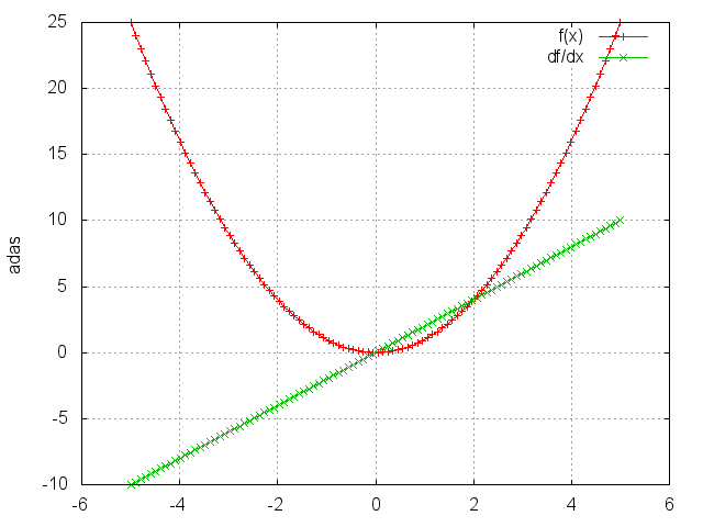
Square
Takes the square of each element.
ii=torch.linspace(-5,5)
m=nn.Square()
oo=m:forward(ii)
go=torch.ones(100)
gi=m:backward(ii,go)
gnuplot.plot({'f(x)',ii,oo,'+-'},{'df/dx',ii,gi,'+-'})
gnuplot.grid(true)
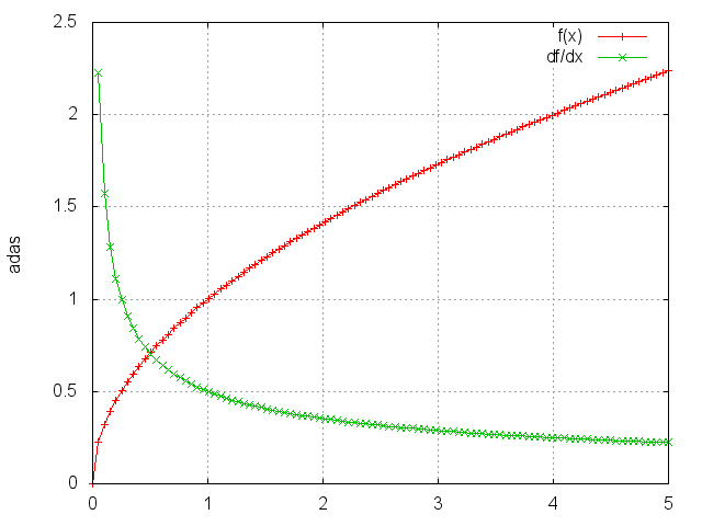
Sqrt
Takes the square root of each element.
ii=torch.linspace(0,5)
m=nn.Sqrt()
oo=m:forward(ii)
go=torch.ones(100)
gi=m:backward(ii,go)
gnuplot.plot({'f(x)',ii,oo,'+-'},{'df/dx',ii,gi,'+-'})
gnuplot.grid(true)
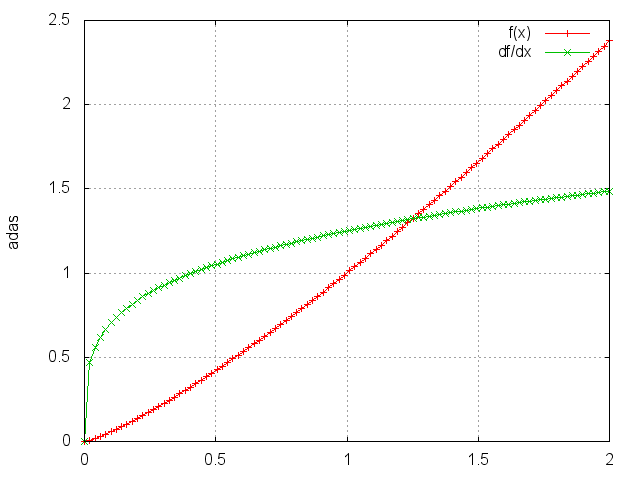
Power
module = Power(p)
Raises each element to its pth power.
ii=torch.linspace(0,2)
m=nn.Power(1.25)
oo=m:forward(ii)
go=torch.ones(100)
gi=m:backward(ii,go)
gnuplot.plot({'f(x)',ii,oo,'+-'},{'df/dx',ii,gi,'+-'})
gnuplot.grid(true)
MM
module = nn.MM(transA, transB)
Performs multiplications on one or more pairs of matrices.
If transA is set, the first matrix is transposed before multiplication.
If transB is set, the second matrix is transposed before multiplication.
By default, the matrices do not get transposed.
The module also accepts 3D inputs which are interpreted as batches of matrices.
When using batches, the first input matrix should be of size b x m x n and the
second input matrix should be of size b x n x p (assuming transA and transB
are not set).
model = nn.MM()
A = torch.randn(b, m, n)
B = torch.randn(b, n, p)
C = model.forward({A, B})  -- C will be of size `b x m x n`