Transfer Function Layers
Transfer functions are normally used to introduce a non-linearity after a parameterized layer like Linear and SpatialConvolution. Non-linearities allows for dividing the problem space into more complex regions than what a simple logistic regressor would permit.
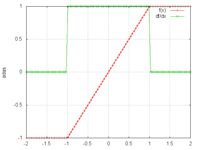
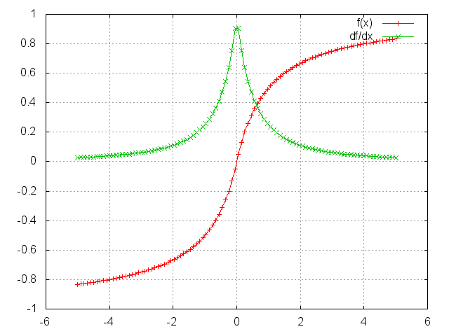
HardTanh
Applies the HardTanh function element-wise to the input Tensor,
thus outputting a Tensor of the same dimension.
HardTanh is defined as:
f(x)=1, if x >1,f(x)=-1, if x <-1,f(x)=x,otherwise.
ii=torch.linspace(-2,2)
m=nn.HardTanh()
oo=m:forward(ii)
go=torch.ones(100)
gi=m:backward(ii,go)
gnuplot.plot({'f(x)',ii,oo,'+-'},{'df/dx',ii,gi,'+-'})
gnuplot.grid(true)
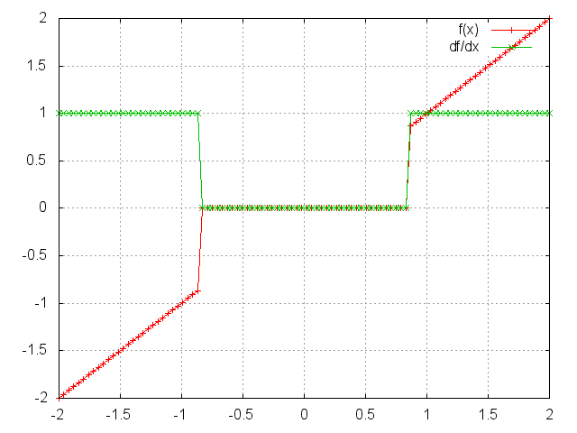
HardShrink
module = nn.HardShrink(lambda)
Applies the hard shrinkage function element-wise to the input Tensor. The output is the same size as the input.
HardShrinkage operator is defined as:
f(x) = x, if x > lambdaf(x) = -x, if x < -lambdaf(x) = 0, otherwise
ii=torch.linspace(-2,2)
m=nn.HardShrink(0.85)
oo=m:forward(ii)
go=torch.ones(100)
gi=m:backward(ii,go)
gnuplot.plot({'f(x)',ii,oo,'+-'},{'df/dx',ii,gi,'+-'})
gnuplot.grid(true)
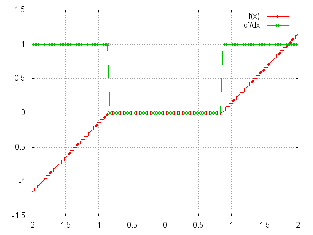
SoftShrink
module = nn.SoftShrink(lambda)
Applies the hard shrinkage function element-wise to the input Tensor. The output is the same size as the input.
HardShrinkage operator is defined as:
f(x) = x-lambda, if x > lambdaf(x) = -x+lambda, if x < -lambdaf(x) = 0, otherwise
ii=torch.linspace(-2,2)
m=nn.SoftShrink(0.85)
oo=m:forward(ii)
go=torch.ones(100)
gi=m:backward(ii,go)
gnuplot.plot({'f(x)',ii,oo,'+-'},{'df/dx',ii,gi,'+-'})
gnuplot.grid(true)
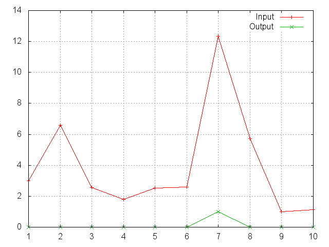
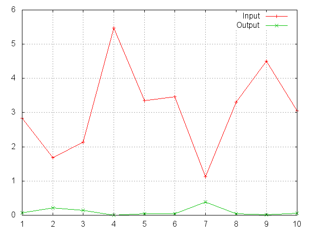
SoftMax
Applies the Softmax function to an n-dimensional input Tensor,
rescaling them so that the elements of the n-dimensional output Tensor
lie in the range (0,1) and sum to 1.
Softmax is defined as f_i(x) = exp(x_i-shift) / sum_j exp(x_j-shift),
where shift = max_i x_i.
ii=torch.exp(torch.abs(torch.randn(10)))
m=nn.SoftMax()
oo=m:forward(ii)
gnuplot.plot({'Input',ii,'+-'},{'Output',oo,'+-'})
gnuplot.grid(true)
Note that this module doesn't work directly with ClassNLLCriterion, which expects the nn.Log to be computed between the SoftMax and itself. Use LogSoftMax instead (it's faster).
SoftMin
Applies the Softmin function to an n-dimensional input Tensor,
rescaling them so that the elements of the n-dimensional output Tensor
lie in the range (0,1) and sum to 1.
Softmin is defined as f_i(x) = exp(-x_i-shift) / sum_j exp(-x_j-shift),
where shift = max_i x_i.
ii=torch.exp(torch.abs(torch.randn(10)))
m=nn.SoftMin()
oo=m:forward(ii)
gnuplot.plot({'Input',ii,'+-'},{'Output',oo,'+-'})
gnuplot.grid(true)
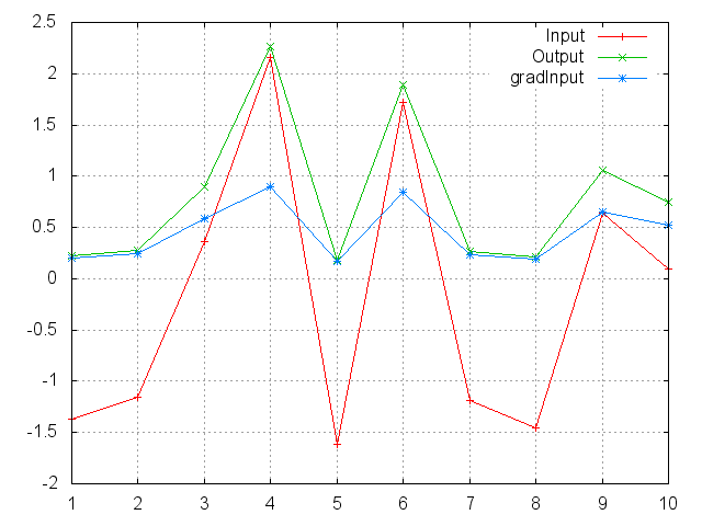
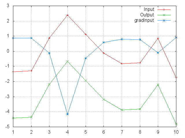
SoftPlus
Applies the SoftPlus function to an n-dimensioanl input Tensor.
Can be used to constrain the output of a machine to always be positive.
SoftPlus is defined as f_i(x) = 1/beta * log(1 + exp(beta * x_i)).
ii=torch.randn(10)
m=nn.SoftPlus()
oo=m:forward(ii)
go=torch.ones(10)
gi=m:backward(ii,go)
gnuplot.plot({'Input',ii,'+-'},{'Output',oo,'+-'},{'gradInput',gi,'+-'})
gnuplot.grid(true)
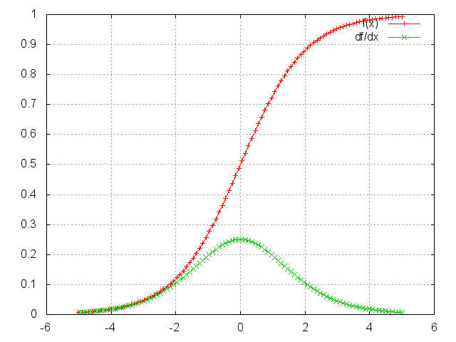
SoftSign
Applies the SoftSign function to an n-dimensioanl input Tensor.
SoftSign is defined as f_i(x) = x_i / (1+|x_i|)
ii=torch.linspace(-5,5)
m=nn.SoftSign()
oo=m:forward(ii)
go=torch.ones(100)
gi=m:backward(ii,go)
gnuplot.plot({'f(x)',ii,oo,'+-'},{'df/dx',ii,gi,'+-'})
gnuplot.grid(true)
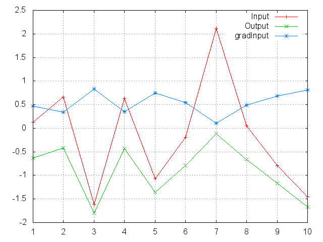
LogSigmoid
Applies the LogSigmoid function to an n-dimensional input Tensor.
LogSigmoid is defined as f_i(x) = log(1/(1+ exp(-x_i))).
ii=torch.randn(10)
m=nn.LogSigmoid()
oo=m:forward(ii)
go=torch.ones(10)
gi=m:backward(ii,go)
gnuplot.plot({'Input',ii,'+-'},{'Output',oo,'+-'},{'gradInput',gi,'+-'})
gnuplot.grid(true)
LogSoftMax
Applies the LogSoftmax function to an n-dimensional input Tensor.
LogSoftmax is defined as f_i(x) = log(1/a exp(x_i)),
where a = sum_j exp(x_j).
ii=torch.randn(10)
m=nn.LogSoftMax()
oo=m:forward(ii)
go=torch.ones(10)
gi=m:backward(ii,go)
gnuplot.plot({'Input',ii,'+-'},{'Output',oo,'+-'},{'gradInput',gi,'+-'})
gnuplot.grid(true)
Sigmoid
Applies the Sigmoid function element-wise to the input Tensor,
thus outputting a Tensor of the same dimension.
Sigmoid is defined as f(x) = 1/(1+exp(-x)).
ii=torch.linspace(-5,5)
m=nn.Sigmoid()
oo=m:forward(ii)
go=torch.ones(100)
gi=m:backward(ii,go)
gnuplot.plot({'f(x)',ii,oo,'+-'},{'df/dx',ii,gi,'+-'})
gnuplot.grid(true)
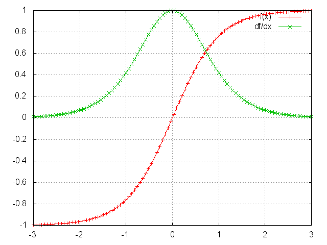
Tanh
Applies the Tanh function element-wise to the input Tensor,
thus outputting a Tensor of the same dimension.
ii=torch.linspace(-3,3)
m=nn.Tanh()
oo=m:forward(ii)
go=torch.ones(100)
gi=m:backward(ii,go)
gnuplot.plot({'f(x)',ii,oo,'+-'},{'df/dx',ii,gi,'+-'})
gnuplot.grid(true)
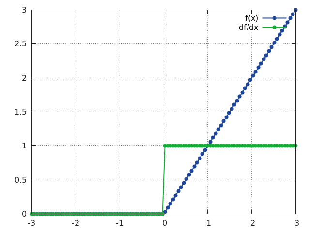
ReLU
Applies the rectified linear unit (ReLU) function element-wise to the input Tensor,
thus outputting a Tensor of the same dimension.
ii=torch.linspace(-3,3)
m=nn.ReLU()
oo=m:forward(ii)
go=torch.ones(100)
gi=m:backward(ii,go)
gnuplot.plot({'f(x)',ii,oo,'+-'},{'df/dx',ii,gi,'+-'})
gnuplot.grid(true)
AddConstant
Adds a (non-learnable) scalar constant. This module is sometimes useful for debuggging purposes: f(x) = x + k, where k is a scalar.
MulConstant
Multiplies input tensor by a (non-learnable) scalar constant. This module is sometimes useful for debuggging purposes: f(x) = k * x, where k is a scalar.