Convolutional layers
A convolution is an integral that expresses the amount of overlap of one function g as it is shifted over another function f. It therefore "blends" one function with another. The neural network package supports convolution, pooling, subsampling and other relevant facilities. These are divided based on the dimensionality of the input and output Tensors:
- Temporal Modules apply to sequences with a one-dimensional relationship
(e.g. sequences of words, phonemes and letters. Strings of some kind).
- TemporalConvolution : a 1D convolution over an input sequence ;
- TemporalSubSampling : a 1D sub-sampling over an input sequence ;
- TemporalMaxPooling : a 1D max-pooling operation over an input sequence ;
- LookupTable : a convolution of width
1, commonly used for word embeddings ; - TemporalRowConvolution : a row-oriented 1D convolution over an input sequence ;
- Spatial Modules apply to inputs with two-dimensional relationships (e.g. images):
- SpatialConvolution : a 2D convolution over an input image ;
- SpatialFullConvolution : a 2D full convolution over an input image ;
- SpatialDilatedConvolution : a 2D dilated convolution over an input image ;
- SpatialDepthWiseConvolution : a 2D depth-wise convolution over an input image ;
- SpatialConvolutionLocal : a 2D locally-connected layer over an input image ;
- SpatialSubSampling : a 2D sub-sampling over an input image ;
- SpatialMaxPooling : a 2D max-pooling operation over an input image ;
- SpatialDilatedMaxPooling : a 2D dilated max-pooling operation over an input image ;
- SpatialFractionalMaxPooling : a 2D fractional max-pooling operation over an input image ;
- SpatialAveragePooling : a 2D average-pooling operation over an input image ;
- SpatialAdaptiveMaxPooling : a 2D max-pooling operation which adapts its parameters dynamically such that the output is of fixed size ;
- SpatialAdaptiveAveragePooling : a 2D average-pooling operation which adapts its parameters dynamically such that the output is of fixed size ;
- SpatialMaxUnpooling : a 2D max-unpooling operation ;
- SpatialLPPooling : computes the
pnorm in a convolutional manner on a set of input images ; - SpatialConvolutionMap : a 2D convolution that uses a generic connection table ;
- SpatialZeroPadding : pads a feature map with specified number of zeros ;
- SpatialReflectionPadding : pads a feature map with the reflection of the input ;
- SpatialReplicationPadding : pads a feature map with the value at the edge of the input borders ;
- SpatialSubtractiveNormalization : a spatial subtraction operation on a series of 2D inputs using
- SpatialCrossMapLRN : a spatial local response normalization between feature maps ;
- SpatialBatchNormalization: mean/std normalization over the mini-batch inputs and pixels, with an optional affine transform that follows a kernel for computing the weighted average in a neighborhood ;
- SpatialUpSamplingNearest: A simple nearest neighbor upsampler applied to every channel of the feature map.
- SpatialUpSamplingBilinear: A simple bilinear upsampler applied to every channel of the feature map.
- Volumetric Modules apply to inputs with three-dimensional relationships (e.g. videos) :
- VolumetricConvolution : a 3D convolution over an input video (a sequence of images) ;
- VolumetricFullConvolution : a 3D full convolution over an input video (a sequence of images) ;
- VolumetricDilatedConvolution : a 3D dilated convolution over an input image ;
- VolumetricMaxPooling : a 3D max-pooling operation over an input video.
- VolumetricDilatedMaxPooling : a 3D dilated max-pooling operation over an input video ;
- VolumetricFractionalMaxPooling : a 3D fractional max-pooling operation over an input image ;
- VolumetricAveragePooling : a 3D average-pooling operation over an input video.
- VolumetricMaxUnpooling : a 3D max-unpooling operation.
- VolumetricReplicationPadding : Pads a volumetric feature map with the value at the edge of the input borders. ;
- UpSampling: Upsampling for either spatial or volumetric inputs using nearest neighbor or linear interpolation.
Temporal Modules
Excluding an optional first batch dimension, temporal layers expect a 2D Tensor as input. The
first dimension is the number of frames in the sequence (e.g. nInputFrame), the last dimension
is the number of features per frame (e.g. inputFrameSize). The output will normally have the same number
of dimensions, although the size of each dimension may change. These are commonly used for processing acoustic signals or sequences of words, i.e. in Natural Language Processing.
Note: The LookupTable is special in that while it does output a temporal Tensor of size nOutputFrame x outputFrameSize,
its input is a 1D Tensor of indices of size nIndices. Again, this is excluding the option first batch dimension.
TemporalConvolution
module = nn.TemporalConvolution(inputFrameSize, outputFrameSize, kW, [dW])
Applies a 1D convolution over an input sequence composed of nInputFrame frames. The input tensor in
forward(input) is expected to be a 2D tensor (nInputFrame x inputFrameSize) or a 3D tensor (nBatchFrame x nInputFrame x inputFrameSize).
The parameters are the following:
* inputFrameSize: The input frame size expected in sequences given into forward().
* outputFrameSize: The output frame size the convolution layer will produce.
* kW: The kernel width of the convolution
* dW: The step of the convolution. Default is 1.
Note that depending of the size of your kernel, several (of the last) frames of the sequence might be lost. It is up to the user to add proper padding frames in the input sequences.
If the input sequence is a 2D tensor of dimension nInputFrame x inputFrameSize, the output sequence will be
nOutputFrame x outputFrameSize where
nOutputFrame = (nInputFrame - kW) / dW + 1
If the input sequence is a 3D tensor of dimension nBatchFrame x nInputFrame x inputFrameSize, the output sequence will be
nBatchFrame x nOutputFrame x outputFrameSize.
The parameters of the convolution can be found in self.weight (Tensor of
size outputFrameSize x (kW x inputFrameSize)) and self.bias (Tensor of
size outputFrameSize). The corresponding gradients can be found in
self.gradWeight and self.gradBias.
For a 2D input, the output value of the layer can be precisely described as:
output[t][i] = bias[i]
  + sum_j sum_{k=1}^kW weight[i][k][j]
                                * input[dW*(t-1)+k)][j]
Here is a simple example:
inp=5;  -- dimensionality of one sequence element
outp=1; -- number of derived features for one sequence element
kw=1;   -- kernel only operates on one sequence element per step
dw=1;   -- we step once and go on to the next sequence element

mlp=nn.TemporalConvolution(inp,outp,kw,dw)

x=torch.rand(7,inp) -- a sequence of 7 elements
print(mlp:forward(x))
which gives:
-0.9109
-0.9872
-0.6808
-0.9403
-0.9680
-0.6901
-0.6387
[torch.Tensor of dimension 7x1]
This is equivalent to:
weights=torch.reshape(mlp.weight,inp) -- weights applied to all
bias= mlp.bias[1];
for i=1,x:size(1) do -- for each sequence element
   element= x[i]; -- features of ith sequence element
   print(element:dot(weights) + bias)
end
which gives:
-0.91094998687717
-0.98721705771773
-0.68075004276185
-0.94030132495887
-0.96798754116609
-0.69008470895581
-0.63871422284166
TemporalMaxPooling
module = nn.TemporalMaxPooling(kW, [dW])
Applies 1D max-pooling operation in kW regions by step size
dW steps. Input sequence composed of nInputFrame frames. The input tensor in
forward(input) is expected to be a 2D tensor (nInputFrame x inputFrameSize)
or a 3D tensor (nBatchFrame x nInputFrame x inputFrameSize).
If the input sequence is a 2D tensor of dimension nInputFrame x inputFrameSize, the output sequence will be
nOutputFrame x inputFrameSize where
nOutputFrame = (nInputFrame - kW) / dW + 1
TemporalSubSampling
module = nn.TemporalSubSampling(inputFrameSize, kW, [dW])
Applies a 1D sub-sampling over an input sequence composed of nInputFrame frames. The input tensor in
forward(input) is expected to be a 2D tensor (nInputFrame x inputFrameSize). The output frame size
will be the same as the input one (inputFrameSize).
The parameters are the following:
* inputFrameSize: The input frame size expected in sequences given into forward().
* kW: The kernel width of the sub-sampling
* dW: The step of the sub-sampling. Default is 1.
Note that depending of the size of your kernel, several (of the last) frames of the sequence might be lost. It is up to the user to add proper padding frames in the input sequences.
If the input sequence is a 2D tensor nInputFrame x inputFrameSize, the output sequence will be
inputFrameSize x nOutputFrame where
nOutputFrame = (nInputFrame - kW) / dW + 1
The parameters of the sub-sampling can be found in self.weight (Tensor of
size inputFrameSize) and self.bias (Tensor of
size inputFrameSize). The corresponding gradients can be found in
self.gradWeight and self.gradBias.
The output value of the layer can be precisely described as:
output[t][i] = bias[i] + weight[i] * sum_{k=1}^kW input[dW*(t-1)+k][i]
LookupTable
module = nn.LookupTable(nIndex, size, [paddingValue], [maxNorm], [normType])
This layer is a particular case of a convolution, where the width of the convolution would be 1.
When calling forward(input), it assumes input is a 1D or 2D tensor filled with indices.
If the input is a matrix, then each row is assumed to be an input sample of given batch. Indices start
at 1 and can go up to nIndex. For each index, it outputs a corresponding Tensor of size
specified by size.
LookupTable can be very slow if a certain input occurs frequently compared to other inputs;
this is often the case for input padding. During the backward step, there is a separate thread
for each input symbol which results in a bottleneck for frequent inputs.
generating a n x size1 x size2 x ... x sizeN tensor, where n
is the size of a 1D input tensor.
Again with a 1D input, when only size1 is provided, the forward(input) is equivalent to
performing the following matrix-matrix multiplication in an efficient manner:
P M
where M is a 2D matrix of size nIndex x size1 containing the parameters of the lookup-table and
P is a 2D matrix of size n x nIndex, where for each ith row vector, every element is zero except the one at index input[i] where it is 1.
1D example:
 -- a lookup table containing 10 tensors of size 3
 module = nn.LookupTable(10, 3)

 input = torch.Tensor{1,2,1,10}
 print(module:forward(input))
Outputs something like:
-1.4415 -0.1001 -0.1708
-0.6945 -0.4350  0.7977
-1.4415 -0.1001 -0.1708
-0.0745  1.9275  1.0915
[torch.DoubleTensor of dimension 4x3]
Note that the first row vector is the same as the 3rd one!
Given a 2D input tensor of size m x n, the output is a m x n x size
tensor, where m is the number of samples in
the batch and n is the number of indices per sample.
2D example:
 -- a lookup table containing 10 tensors of size 3
 module = nn.LookupTable(10, 3)

 -- a batch of 2 samples of 4 indices each
 input = torch.Tensor({{1,2,4,5},{4,3,2,10}})
 print(module:forward(input))
Outputs something like:
(1,.,.) =
 -0.0570 -1.5354  1.8555
 -0.9067  1.3392  0.6275
  1.9662  0.4645 -0.8111
  0.1103  1.7811  1.5969

(2,.,.) =
  1.9662  0.4645 -0.8111
  0.0026 -1.4547 -0.5154
 -0.9067  1.3392  0.6275
 -0.0193 -0.8641  0.7396
[torch.DoubleTensor of dimension 2x4x3]
LookupTable supports max-norm regularization. One can activate the max-norm constraints by setting non-nil maxNorm in constructor or using setMaxNorm function. In the implementation, the max-norm constraint is enforced in the forward pass. That is the output of the LookupTable always obeys the max-norm constraint, even though the module weights may temporarily exceed the max-norm constraint.
max-norm regularization example:
 -- a lookup table with max-norm constraint: 2-norm <= 1
 module = nn.LookupTable(10, 3, 0, 1, 2)
 input = torch.Tensor{1,2,1,10}
 print(module.weight)
 -- output of the module always obey max-norm constraint
 print(module:forward(input))
 -- the rows accessed should be re-normalized
 print(module.weight)
Outputs something like:
 0.2194  1.4759 -1.1829
 0.7069  0.2436  0.9876
-0.2955  0.3267  1.1844
-0.0575 -0.2957  1.5079
-0.2541  0.5331 -0.0083
 0.8005 -1.5994 -0.4732
-0.0065  2.3441 -0.6354
 0.2910  0.4230  0.0975
 1.2662  1.1846  1.0114
-0.4095 -1.0676 -0.9056
[torch.DoubleTensor of size 10x3]

 0.1152  0.7751 -0.6212
 0.5707  0.1967  0.7973
 0.1152  0.7751 -0.6212
-0.2808 -0.7319 -0.6209
[torch.DoubleTensor of size 4x3]

 0.1152  0.7751 -0.6212
 0.5707  0.1967  0.7973
-0.2955  0.3267  1.1844
-0.0575 -0.2957  1.5079
-0.2541  0.5331 -0.0083
 0.8005 -1.5994 -0.4732
-0.0065  2.3441 -0.6354
 0.2910  0.4230  0.0975
 1.2662  1.1846  1.0114
-0.2808 -0.7319 -0.6209
[torch.DoubleTensor of size 10x3]
Note that the 1st, 2nd and 10th rows of the module.weight are updated to obey the max-norm constraint, since their indices appear in the "input".
TemporalRowConvolution
module = nn.TemporalRowConvolution(inputFrameSize, kW, [dW], [featFirst]))
Applies a 1D row-oriented convolution over an input sequence composed of nInputFrame frames. The input tensor in forward(input) is expected to be a 2D tensor (nInputFrame x inputFrameSize) or a 3D tensor (nBatchFrame x nInputFrame x inputFrameSize). The layer can be used without a bias by module:noBias().
The parameters are the following:
* inputFrameSize: The input frame size expected in sequences given into forward().
* kW: The kernel width of the convolution.
* dW: The step of the convolution Default is 1.
* featFirst: Expects input to be in the form nBatchFrame x inputFrameSize x nInputFrame is true. Default is false.
If the input sequence is a 2D tensor of dimension nInputFrame x inputFrameSize, the output sequence will be nOutputFrame x inputFrameSize where
lua
  nOutputFrame = (nInputFrame - kW) / dW + 1
If the input sequence is a 3D tensor of dimension nBatchFrame x nInputFrame x inputFrameSize, the output sequence will be nBatch x nOutputFrame x outputFrameSize.
The parameters are the convolution can be found in self.weight (Tensor of size inputFrameSize x kW) and self.bias (Tensor of size inputFrameSize). The corresponding gradients can be found in self.gradWeight and self.gradBias.
For a 2D input, the output value of the layer can be precisely described as:
lua
  output[t][i] = bias[i] + sum_{k=1}^kW weight[i][k] * input[dW(t-1)+k][i]
Here is a simple example: ```lua inp = 5; kw = 3; dw = 1;
-- row convolution with a kernel width of 3 (future context of 2) module = nn.TemporalRowConvolution(inp, kw, dw)
x = torch.rand(8, inp) print(module:forward(x)) ```
which gives
lua
  0.1188  0.1945  0.1065 -0.0077 -0.3433
  0.0630  0.4354  0.1954 -0.2103 -0.3506
  0.0340  0.2222  0.3039 -0.2012 -0.3814
  0.0820  0.3489  0.2533 -0.0940 -0.3298
  0.1964  0.1533  0.1750 -0.1493 -0.3059
  0.2651  0.2474  0.0521 -0.1134 -0.4024
  [torch.Tensor of dimension 8x5]
More information about the layer can be found here.
Spatial Modules
Excluding an optional batch dimension, spatial layers expect a 3D Tensor as input. The
first dimension is the number of features (e.g. frameSize), the last two dimensions
are spatial (e.g. height x width). These are commonly used for processing images.
SpatialConvolution
module = nn.SpatialConvolution(nInputPlane, nOutputPlane, kW, kH, [dW], [dH], [padW], [padH])
Applies a 2D convolution over an input image composed of several input planes. The input tensor in
forward(input) is expected to be a 3D tensor (nInputPlane x height x width).
The parameters are the following:
* nInputPlane: The number of expected input planes in the image given into forward().
* nOutputPlane: The number of output planes the convolution layer will produce.
* kW: The kernel width of the convolution
* kH: The kernel height of the convolution
* dW: The step of the convolution in the width dimension. Default is 1.
* dH: The step of the convolution in the height dimension. Default is 1.
* padW: Additional zeros added to the input plane data on both sides of width axis. Default is 0. (kW-1)/2 is often used here.
* padH: Additional zeros added to the input plane data on both sides of height axis. Default is 0. (kH-1)/2 is often used here.
Note that depending of the size of your kernel, several (of the last) columns or rows of the input image might be lost. It is up to the user to add proper padding in images.
If the input image is a 3D tensor nInputPlane x height x width, the output image size
will be nOutputPlane x oheight x owidth where
owidth  = floor((width  + 2*padW - kW) / dW + 1)
oheight = floor((height + 2*padH - kH) / dH + 1)
The parameters of the convolution can be found in self.weight (Tensor of
size nOutputPlane x nInputPlane x kH x kW) and self.bias (Tensor of
size nOutputPlane). The corresponding gradients can be found in
self.gradWeight and self.gradBias.
The output value of the layer can be precisely described as:
output[i][j][k] = bias[k]
  + sum_l sum_{s=1}^kW sum_{t=1}^kH weight[s][t][l][k]
                                    * input[dW*(i-1)+s)][dH*(j-1)+t][l]
SpatialConvolutionMap
module = nn.SpatialConvolutionMap(connectionMatrix, kW, kH, [dW], [dH])
This class is a generalization of nn.SpatialConvolution. It uses a generic connection table between input and output features. The nn.SpatialConvolution is equivalent to using a full connection table. One can specify different types of connection tables.
Full Connection Table
table = nn.tables.full(nin,nout)
This is a precomputed table that specifies connections between every input and output node.
One to One Connection Table
table = nn.tables.oneToOne(n)
This is a precomputed table that specifies a single connection to each output node from corresponding input node.
Random Connection Table
table = nn.tables.random(nin,nout, nto)
This table is randomly populated such that each output unit has
nto incoming connections. The algorithm tries to assign uniform
number of outgoing connections to each input node if possible.
SpatialFullConvolution
module = nn.SpatialFullConvolution(nInputPlane, nOutputPlane, kW, kH, [dW], [dH], [padW], [padH], [adjW], [adjH])
Applies a 2D full convolution over an input image composed of several input planes. The input tensor in
forward(input) is expected to be a 3D or 4D tensor. Note that instead of setting adjW and adjH, SpatialFullConvolution also accepts a table input with two tensors: {convInput, sizeTensor} where convInput is the standard input on which the full convolution
is applied, and the size of sizeTensor is used to set the size of the output. Using the two-input version of forward
will ignore the adjW and adjH values used to construct the module. The layer can be used without a bias by module:noBias().
Other frameworks call this operation "In-network Upsampling", "Fractionally-strided convolution", "Backwards Convolution," "Deconvolution", or "Upconvolution."
The parameters are the following:
* nInputPlane: The number of expected input planes in the image given into forward().
* nOutputPlane: The number of output planes the convolution layer will produce.
* kW: The kernel width of the convolution
* kH: The kernel height of the convolution
* dW: The step of the convolution in the width dimension. Default is 1.
* dH: The step of the convolution in the height dimension. Default is 1.
* padW: Additional zeros added to the input plane data on both sides of width axis. Default is 0. (kW-1)/2 is often used here.
* padH: Additional zeros added to the input plane data on both sides of height axis. Default is 0. (kH-1)/2 is often used here.
* adjW: Extra width to add to the output image. Default is 0. Cannot be greater than dW-1.
* adjH: Extra height to add to the output image. Default is 0. Cannot be greater than dH-1.
If the input image is a 3D tensor nInputPlane x height x width, the output image size
will be nOutputPlane x oheight x owidth where
owidth  = (width  - 1) * dW - 2*padW + kW + adjW
oheight = (height - 1) * dH - 2*padH + kH + adjH
Further information about the full convolution can be found in the following paper: Fully Convolutional Networks for Semantic Segmentation.
SpatialDilatedConvolution
module = nn.SpatialDilatedConvolution(nInputPlane, nOutputPlane, kW, kH, [dW], [dH], [padW], [padH], [dilationW], [dilationH])
Also sometimes referred to as atrous convolution.
Applies a 2D dilated convolution over an input image composed of several input planes. The input tensor in
forward(input) is expected to be a 3D or 4D tensor.
The parameters are the following:
* nInputPlane: The number of expected input planes in the image given into forward().
* nOutputPlane: The number of output planes the convolution layer will produce.
* kW: The kernel width of the convolution
* kH: The kernel height of the convolution
* dW: The step of the convolution in the width dimension. Default is 1.
* dH: The step of the convolution in the height dimension. Default is 1.
* padW: Additional zeros added to the input plane data on both sides of width axis. Default is 0. (kW-1)/2 is often used here.
* padH: Additional zeros added to the input plane data on both sides of height axis. Default is 0. (kH-1)/2 is often used here.
* dilationW: The number of pixels to skip. Default is 1. 1 makes it a SpatialConvolution
* dilationH: The number of pixels to skip. Default is 1. 1 makes it a SpatialConvolution
If the input image is a 3D tensor nInputPlane x height x width, the output image size
will be nOutputPlane x oheight x owidth where
owidth  = floor((width + 2 * padW - dilationW * (kW-1) - 1) / dW) + 1
oheight = floor((height + 2 * padH - dilationH * (kH-1) - 1) / dH) + 1
Further information about the dilated convolution can be found in the following paper: Multi-Scale Context Aggregation by Dilated Convolutions.
SpatialDepthWiseConvolution
module = nn.SpatialDepthWiseConvolution(nInputPlane, nOutputPlane, kW, kH, [dW], [dH], [padW], [padH])
Applies a 2D depth-wise convolution over an input image composed of several input planes. The input tensor in
forward(input) is expected to be a 3D tensor (nInputPlane x height x width).
It is similar to SpatialConvolution, but here a spatial convolution is performed independently over each channel of an input. The most noticiable difference is the output dimension of SpatialConvolution is nOutputPlane x oheight x owidth, while for SpatialDepthWiseConvolution it is (nOutputPlane x nInputPlane) x oheight x owidth.
The parameters are the following:
* nInputPlane: The number of expected input planes in the image given into forward().
* nOutputPlane: The number of output planes the convolution layer will produce.
* kW: The kernel width of the convolution
* kH: The kernel height of the convolution
* dW: The step of the convolution in the width dimension. Default is 1.
* dH: The step of the convolution in the height dimension. Default is 1.
* padW: Additional zeros added to the input plane data on both sides of width axis. Default is 0. (kW-1)/2 is often used here.
* padH: Additional zeros added to the input plane data on both sides of height axis. Default is 0. (kH-1)/2 is often used here.
Note that depending of the size of your kernel, several (of the last) columns or rows of the input image might be lost. It is up to the user to add proper padding in images.
If the input image is a 3D tensor nInputPlane x height x width, the output image size
will be a 3D tensor (nOutputPlane x nInputPlane) x oheight x owidth where
owidth  = floor((width  + 2*padW - kW) / dW + 1)
oheight = floor((height + 2*padH - kH) / dH + 1)
The parameters of the convolution can be found in self.weight (Tensor of
size nOutputPlane x nInputPlane x kH x kW) and self.bias (Tensor of
size nOutputPlane x nInputPlane). The corresponding gradients can be found in
self.gradWeight and self.gradBias.
The output value of the layer can be described as:
output[i][j] = input[j] * weight[i][j] + b[i][j], i = 1, ..., nOutputPlane, j = 1, ..., nInputPlane
Further information about the dilated convolution can be found in the following paper: Xception: Deep Learning with Depthwise Separable Convolutions.
SpatialConvolutionLocal
module = nn.SpatialConvolutionLocal(nInputPlane, nOutputPlane, iW, iH, kW, kH, [dW], [dH], [padW], [padH])
Applies a 2D locally-connected layer over an input image composed of several input planes. The input tensor in
forward(input) is expected to be a 3D or 4D tensor.
A locally-connected layer is similar to a convolution layer but without weight-sharing.
The parameters are the following:
* nInputPlane: The number of expected input planes in the image given into forward().
* nOutputPlane: The number of output planes the locally-connected layer will produce.
* iW: The input width.
* iH: The input height.
* kW: The kernel width.
* kH: The kernel height.
* dW: The step in the width dimension. Default is 1.
* dH: The step in the height dimension. Default is 1.
* padW: Additional zeros added to the input plane data on both sides of width axis. Default is 0.
* padH: Additional zeros added to the input plane data on both sides of height axis. Default is 0.
If the input image is a 3D tensor nInputPlane x iH x iW, the output image size
will be nOutputPlane x oH x oW where
oW  = floor((iW  + 2*padW - kW) / dW + 1)
oH = floor((iH + 2*padH - kH) / dH + 1)
SpatialLPPooling
module = nn.SpatialLPPooling(nInputPlane, pnorm, kW, kH, [dW], [dH])
Computes the p norm in a convolutional manner on a set of 2D input planes.
SpatialMaxPooling
module = nn.SpatialMaxPooling(kW, kH [, dW, dH, padW, padH])
Applies 2D max-pooling operation in kWxkH regions by step size
dWxdH steps. The number of output features is equal to the number of
input planes.
If the input image is a 3D tensor nInputPlane x height x width, the output
image size will be nOutputPlane x oheight x owidth where
owidth  = op((width  + 2*padW - kW) / dW + 1)
oheight = op((height + 2*padH - kH) / dH + 1)
op is a rounding operator. By default, it is floor. It can be changed
by calling :ceil() or :floor() methods.
SpatialDilatedMaxPooling
module = nn.SpatialDilatedMaxPooling(kW, kH [, dW, dH, padW, padH, dilationW, dilationH])
Also sometimes referred to as atrous pooling.
Applies 2D dilated max-pooling operation in kWxkH regions by step size
dWxdH steps. The number of output features is equal to the number of
input planes. If dilationW and dilationH are not provided, this is equivalent to performing normal nn.SpatialMaxPooling.
If the input image is a 3D tensor nInputPlane x height x width, the output
image size will be nOutputPlane x oheight x owidth where
owidth  = op((width - (dilationW * (kW - 1) + 1) + 2*padW) / dW + 1)
oheight = op((height - (dilationH * (kH - 1) + 1) + 2*padH) / dH + 1)
op is a rounding operator. By default, it is floor. It can be changed
by calling :ceil() or :floor() methods.
SpatialFractionalMaxPooling
module = nn.SpatialFractionalMaxPooling(kW, kH, outW, outH)
--   the output should be the exact size (outH x outW)
OR
module = nn.SpatialFractionalMaxPooling(kW, kH, ratioW, ratioH)
--   the output should be the size (floor(inH x ratioH) x floor(inW x ratioW))
--   ratios are numbers between (0, 1) exclusive
Applies 2D Fractional max-pooling operation as described in the paper "Fractional Max Pooling" by Ben Graham in the "pseudorandom" mode.
The max-pooling operation is applied in kWxkH regions by a stochastic step size determined by the target output size.
The number of output features is equal to the number of input planes.
There are two constructors available.
Constructor 1:
module = nn.SpatialFractionalMaxPooling(kW, kH, outW, outH)
Constructor 2:
module = nn.SpatialFractionalMaxPooling(kW, kH, ratioW, ratioH)
If the input image is a 3D tensor nInputPlane x height x width, the output
image size will be nOutputPlane x oheight x owidth
where
owidth  = floor(width * ratioW)
oheight = floor(height * ratioH)
ratios are numbers between (0, 1) exclusive
SpatialAveragePooling
module = nn.SpatialAveragePooling(kW, kH [, dW, dH, padW, padH])
Applies 2D average-pooling operation in kWxkH regions by step size
dWxdH steps. The number of output features is equal to the number of
input planes.
If the input image is a 3D tensor nInputPlane x height x width, the output
image size will be nOutputPlane x oheight x owidth where
owidth  = op((width  + 2*padW - kW) / dW + 1)
oheight = op((height + 2*padH - kH) / dH + 1)
op is a rounding operator. By default, it is floor. It can be changed
by calling :ceil() or :floor() methods.
By default, the output of each pooling region is divided by the number of
elements inside the padded image (which is usually kW*kH, except in some
corner cases in which it can be smaller). You can also divide by the number
of elements inside the original non-padded image. To switch between different
division factors, call :setCountIncludePad() or :setCountExcludePad(). If
padW=padH=0, both options give the same results.
SpatialAdaptiveMaxPooling
module = nn.SpatialAdaptiveMaxPooling(W, H)
Applies 2D max-pooling operation in an image such that the output is of
size WxH, for any input size. The number of output features is equal
to the number of input planes.
For an output of dimensions (owidth,oheight), the indexes of the pooling
region (j,i) in the input image of dimensions (iwidth,iheight) are
given by:
x_j_start = floor((j   /owidth)  * iwidth)
x_j_end   = ceil(((j+1)/owidth)  * iwidth)

y_i_start = floor((i   /oheight) * iheight)
y_i_end   = ceil(((i+1)/oheight) * iheight)
SpatialAdaptiveAveragePooling
module = nn.SpatialAdaptiveAveragePooling(W, H)
Applies 2D average-pooling operation in an image such that the output is of
size WxH, for any input size. The number of output features is equal
to the number of input planes.
The pooling region algorithm is the same as that in SpatialAdaptiveMaxPooling.
SpatialMaxUnpooling
module = nn.SpatialMaxUnpooling(poolingModule)
Applies 2D "max-unpooling" operation using the indices previously computed
by the SpatialMaxPooling module poolingModule.
When B = poolingModule:forward(A) is called, the indices of the maximal
values (corresponding to their position within each map) are stored:
B[{n,k,i,j}] = A[{n,k,indices[{n,k,i}],indices[{n,k,j}]}].
If C is a tensor of same size as B, module:updateOutput(C) outputs a
tensor D of same size as A such that:
D[{n,k,indices[{n,k,i}],indices[{n,k,j}]}] = C[{n,k,i,j}].
Module inspired by: "Visualizing and understanding convolutional networks" (2014) by Matthew Zeiler, Rob Fergus
SpatialSubSampling
module = nn.SpatialSubSampling(nInputPlane, kW, kH, [dW], [dH])
Applies a 2D sub-sampling over an input image composed of several input planes. The input tensor in
forward(input) is expected to be a 3D tensor (nInputPlane x height x width). The number of output
planes will be the same as nInputPlane.
The parameters are the following:
* nInputPlane: The number of expected input planes in the image given into forward().
* kW: The kernel width of the sub-sampling
* kH: The kernel height of the sub-sampling
* dW: The step of the sub-sampling in the width dimension. Default is 1.
* dH: The step of the sub-sampling in the height dimension. Default is 1.
Note that depending of the size of your kernel, several (of the last) columns or rows of the input image might be lost. It is up to the user to add proper padding in images.
If the input image is a 3D tensor nInputPlane x height x width, the output image size
will be nInputPlane x oheight x owidth where
owidth  = (width  - kW) / dW + 1
oheight = (height - kH) / dH + 1 .
The parameters of the sub-sampling can be found in self.weight (Tensor of
size nInputPlane) and self.bias (Tensor of size nInputPlane). The
corresponding gradients can be found in self.gradWeight and
self.gradBias.
The output value of the layer can be precisely described as:
output[i][j][k] = bias[k]
  + weight[k] sum_{s=1}^kW sum_{t=1}^kH input[dW*(i-1)+s)][dH*(j-1)+t][k]
SpatialUpSamplingNearest
module = nn.SpatialUpSamplingNearest(scale)
Applies a 2D up-sampling over an input image composed of several input planes. The input tensor in
forward(input) is expected to be a 3D or 4D tensor (i.e. for 4D: nBatchPlane x nInputPlane x height x width). The number of output planes will be the same. The v dimension is assumed to be the second last dimension (i.e. for 4D it will be the 3rd dim), and the u dimension is assumed to be the last dimension.
The parameters are the following:
* scale: The upscale ratio. Must be a positive integer
The up-scaling method is simple nearest neighbor, ie:
output(u,v) = input(floor((u-1)/scale)+1, floor((v-1)/scale)+1)
Where u and v are index from 1 (as per lua convention). There are no learnable parameters.
SpatialUpSamplingBilinear
module = nn.SpatialUpSamplingBilinear(scale)
module = nn.SpatialUpSamplingBilinear({oheight=H, owidth=W})
Applies a 2D up-sampling over an input image composed of several input planes. The input tensor in
forward(input) is expected to be a 3D or 4D tensor (i.e. for 4D: nBatchPlane x nInputPlane x height x width). The number of output planes will be the same. The v dimension is assumed to be the second last dimension (i.e. for 4D it will be the 3rd dim), and the u dimension is assumed to be the last dimension.
The parameters are the following:
* scale: The upscale ratio. Must be a positive integer
* Or a table {oheight=H, owidth=W}: The required output height and width, should be positive integers.
The up-scaling method is bilinear.
If scale is specified, given an input of height iH and width iW, output height and width will be:
oH = (iH - 1)(scale - 1) + iH
oW = (iW - 1)(scale - 1) + iW
There are no learnable parameters.
SpatialZeroPadding
module = nn.SpatialZeroPadding(padLeft, padRight, padTop, padBottom)
Each feature map of a given input is padded with specified number of zeros. If padding values are negative, then input is cropped.
SpatialReflectionPadding
module = nn.SpatialReflectionPadding(padLeft, padRight, padTop, padBottom)
Each feature map of a given input is padded with the reflection of the input boundary
SpatialReplicationPadding
module = nn.SpatialReplicationPadding(padLeft, padRight, padTop, padBottom)
Each feature map of a given input is padded with the replication of the input boundary
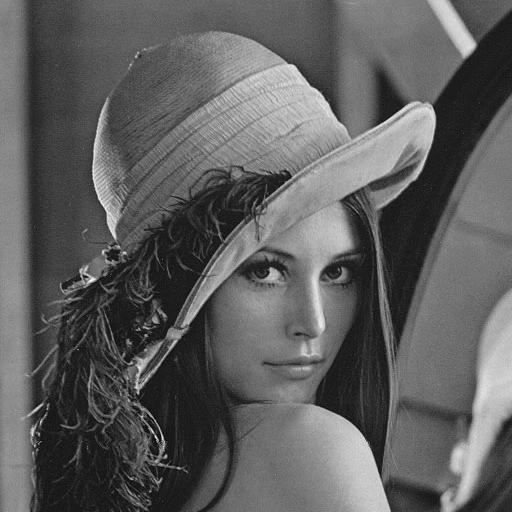
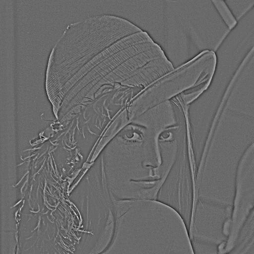
SpatialSubtractiveNormalization
module = nn.SpatialSubtractiveNormalization(ninputplane, kernel)
Applies a spatial subtraction operation on a series of 2D inputs using
kernel for computing the weighted average in a neighborhood. The
neighborhood is defined for a local spatial region that is the size as
kernel and across all features. For a an input image, since there is
only one feature, the region is only spatial. For an RGB image, the
weighted average is taken over RGB channels and a spatial region.
If the kernel is 1D, then it will be used for constructing and seperable
2D kernel. The operations will be much more efficient in this case.
The kernel is generally chosen as a gaussian when it is believed that the correlation of two pixel locations decrease with increasing distance. On the feature dimension, a uniform average is used since the weighting across features is not known.
For this example we use an external package image
require 'image'
require 'nn'
lena = image.rgb2y(image.lena())
ker = torch.ones(11)
m=nn.SpatialSubtractiveNormalization(1,ker)
processed = m:forward(lena)
w1=image.display(lena)
w2=image.display(processed)
SpatialCrossMapLRN
module = nn.SpatialCrossMapLRN(size [,alpha] [,beta] [,k])
Applies Spatial Local Response Normalization between different feature maps.
By default, alpha = 0.0001, beta = 0.75 and k = 1
The operation implemented is:
                          x_f
y_f =  -------------------------------------------------
        (k+(alpha/size)* sum_{l=l1 to l2} (x_l^2))^beta
where x_f is the input at spatial locations h,w (not shown for simplicity) and feature map f,
l1 corresponds to max(0,f-ceil(size/2)) and l2 to min(F, f-ceil(size/2) + size). Here, F
is the number of feature maps.
More information can be found here.
SpatialBatchNormalization
module = nn.SpatialBatchNormalization(N [,eps] [, momentum] [,affine])
where N = number of input feature maps
eps is a small value added to the standard-deviation to avoid divide-by-zero. Defaults to 1e-5
affine is a boolean. When set to false, the learnable affine transform is disabled. Defaults to true
Implements Batch Normalization as described in the paper: "Batch Normalization: Accelerating Deep Network Training by Reducing Internal Covariate Shift" by Sergey Ioffe, Christian Szegedy
The operation implemented is:
   y =     ( x - mean(x) )
        -------------------- * gamma + beta
       standard-deviation(x)
where the mean and standard-deviation are calculated per feature-map over the mini-batches and pixels and where gamma and beta are learnable parameter vectors of size N (where N = number of feature maps). The learning of gamma and beta is optional.
In training time, this layer keeps a running estimate of it's computed mean and std. The running sum is kept with a default momentup of 0.1 (unless over-ridden) In test time, this running mean/std is used to normalize. (Note that the running mean/std will not be saved if one only checkpoints a model's parameters. In order to correctly use the calculated running mean/std, one needs to checkpoint the model itself (call clearState() first to save space).)
The module only accepts 4D inputs.
-- with learnable parameters
model = nn.SpatialBatchNormalization(m)
A = torch.randn(b, m, h, w)
C = model:forward(A)  -- C will be of size `b x m x h x w`

-- without learnable parameters
model = nn.SpatialBatchNormalization(m, nil, nil, false)
A = torch.randn(b, m, h, w)
C = model:forward(A)  -- C will be of size `b x m x h x w`
Volumetric Modules
Excluding an optional batch dimension, volumetric layers expect a 4D Tensor as input. The
first dimension is the number of features (e.g. frameSize), the second is sequential (e.g. time) and the
last two dimensions are spatial (e.g. height x width). These are commonly used for processing videos (sequences of images).
VolumetricConvolution
module = nn.VolumetricConvolution(nInputPlane, nOutputPlane, kT, kW, kH [, dT, dW, dH, padT, padW, padH])
Applies a 3D convolution over an input image composed of several input planes. The input tensor in
forward(input) is expected to be a 4D tensor (nInputPlane x time x height x width).
The parameters are the following:
* nInputPlane: The number of expected input planes in the image given into forward().
* nOutputPlane: The number of output planes the convolution layer will produce.
* kT: The kernel size of the convolution in time
* kW: The kernel width of the convolution
* kH: The kernel height of the convolution
* dT: The step of the convolution in the time dimension. Default is 1.
* dW: The step of the convolution in the width dimension. Default is 1.
* dH: The step of the convolution in the height dimension. Default is 1.
* padT: Additional zeros added to the input plane data on both sides of time axis. Default is 0. (kT-1)/2 is often used here.
* padW: Additional zeros added to the input plane data on both sides of width axis. Default is 0. (kW-1)/2 is often used here.
* padH: Additional zeros added to the input plane data on both sides of height axis. Default is 0. (kH-1)/2 is often used here.
Note that depending of the size of your kernel, several (of the last) columns or rows of the input image might be lost. It is up to the user to add proper padding in images. This layer can be used without a bias by module:noBias().
If the input image is a 4D tensor nInputPlane x time x height x width, the output image size
will be nOutputPlane x otime x oheight x owidth where
otime  = floor((time  + 2*padT - kT) / dT + 1)
owidth  = floor((width  + 2*padW - kW) / dW + 1)
oheight  = floor((height  + 2*padH - kH) / dH + 1)
The parameters of the convolution can be found in self.weight (Tensor of
size nOutputPlane x nInputPlane x kT x kH x kW) and self.bias (Tensor of
size nOutputPlane). The corresponding gradients can be found in
self.gradWeight and self.gradBias.
VolumetricFullConvolution
module = nn.VolumetricFullConvolution(nInputPlane, nOutputPlane, kT, kW, kH, [dT], [dW], [dH], [padT], [padW], [padH], [adjT], [adjW], [adjH])
Applies a 3D full convolution over an input image composed of several input planes. The input tensor in
forward(input) is expected to be a 4D or 5D tensor. Note that instead of setting adjT, adjW and adjH, VolumetricFullConvolution also accepts a table input with two tensors: {convInput, sizeTensor} where convInput is the standard input on which the full convolution is applied, and the size of sizeTensor is used to set the size of the output. Using the two-input version of forward
will ignore the adjT, adjW and adjH values used to construct the module.
This can be used as 3D deconvolution, or 3D upsampling. So that the 3D FCN can be easly implemented. This layer can be used without a bias by module:noBias().
The parameters are the following:
nInputPlane: The number of expected input planes in the image given into forward().
nOutputPlane: The number of output planes the convolution layer will produce.
kT: The kernel depth of the convolution
kW: The kernel width of the convolution
kH: The kernel height of the convolution
dT: The step of the convolution in the depth dimension. Default is 1.
dW: The step of the convolution in the width dimension. Default is 1.
dH: The step of the convolution in the height dimension. Default is 1.
padT: Additional zeros added to the input plane data on both sides of time (depth) axis. Default is 0. (kT-1)/2 is often used here.
padW: Additional zeros added to the input plane data on both sides of width axis. Default is 0. (kW-1)/2 is often used here.
padH: Additional zeros added to the input plane data on both sides of height axis. Default is 0. (kH-1)/2 is often used here.
adjT: Extra depth to add to the output image. Default is 0. Cannot be greater than dT-1.
adjW: Extra width to add to the output image. Default is 0. Cannot be greater than dW-1.
adjH: Extra height to add to the output image. Default is 0. Cannot be greater than dH-1.
If the input image is a 3D tensor nInputPlane x depth x height x width, the output image size
will be nOutputPlane x odepth x oheight x owidth where
odepth  = (depth  - 1) * dT - 2*padT + kT + adjT
owidth  = (width  - 1) * dW - 2*padW + kW + adjW
oheight = (height - 1) * dH - 2*padH + kH + adjH
VolumetricDilatedConvolution
module = nn.VolumetricDilatedConvolution(nInputPlane, nOutputPlane, kT, kW, kH, [dT], [dW], [dH], [padT], [padW], [padH], [dilationT], [dilationW], [dilationH])
Applies a 3D dilated convolution over an input image composed of several input planes. The input tensor in
forward(input) is expected to be a 4D or 5D tensor.
The parameters are the following:
* nInputPlane: The number of expected input planes in the image given into forward().
* nOutputPlane: The number of output planes the convolution layer will produce.
* kT: The kernel depth of the convolution
* kW: The kernel width of the convolution
* kH: The kernel height of the convolution
* dT: The step of the convolution in the depth dimension. Default is 1.
* dW: The step of the convolution in the width dimension. Default is 1.
* dH: The step of the convolution in the height dimension. Default is 1.
* padT: Additional zeros added to the input plane data on both sides of time (depth) axis. Default is 0. (kT-1)/2 is often used here.
* padW: Additional zeros added to the input plane data on both sides of width axis. Default is 0. (kW-1)/2 is often used here.
* padH: Additional zeros added to the input plane data on both sides of height axis. Default is 0. (kH-1)/2 is often used here.
* dilationT: The number of pixels to skip. Default is 1. 1 makes it a VolumetricConvolution
* dilationW: The number of pixels to skip. Default is 1. 1 makes it a VolumetricConvolution
* dilationH: The number of pixels to skip. Default is 1. 1 makes it a VolumetricConvolution
If the input image is a 4D tensor nInputPlane x depth x height x width, the output image size
will be nOutputPlane x odepth x oheight x owidth where
odepth  = floor((depth + 2 * padT - dilationT * (kT-1) + 1) / dT) + 1
owidth  = floor((width + 2 * padW - dilationW * (kW-1) + 1) / dW) + 1
oheight = floor((height + 2 * padH - dilationH * (kH-1) + 1) / dH) + 1
Further information about the dilated convolution can be found in the following paper: Multi-Scale Context Aggregation by Dilated Convolutions.
VolumetricMaxPooling
module = nn.VolumetricMaxPooling(kT, kW, kH [, dT, dW, dH, padT, padW, padH])
Applies 3D max-pooling operation in kTxkWxkH regions by step size
dTxdWxdH steps. The number of output features is equal to the number of
input planes / dT. The input can optionally be padded with zeros. Padding should be smaller than half of kernel size. That is, padT < kT/2, padW < kW/2 and padH < kH/2.
VolumetricDilatedMaxPooling
module = nn.VolumetricDilatedMaxPooling(kT, kW, kH [, dT, dW, dH, padT, padW, padH, dilationT, dilationW, dilationH])
Also sometimes referred to as atrous pooling.
Applies 3D dilated max-pooling operation in kTxkWxkH regions by step size
dTxdWxdH steps. The number of output features is equal to the number of
input planes. If dilationT, dilationW and dilationH are not provided, this is equivalent to performing normal nn.VolumetricMaxPooling.
If the input image is a 4D tensor nInputPlane x depth x height x width, the output
image size will be nOutputPlane x otime x oheight x owidth where
otime  = op((depth - (dilationT * (kT - 1) + 1) + 2*padT) / dT + 1)
owidth  = op((width - (dilationW * (kW - 1) + 1) + 2*padW) / dW + 1)
oheight = op((height - (dilationH * (kH - 1) + 1) + 2*padH) / dH + 1)
op is a rounding operator. By default, it is floor. It can be changed
by calling :ceil() or :floor() methods.
VolumetricFractionalMaxPooling
module = nn.VolumetricFractionalMaxPooling(kT, kW, kH, outT, outW, outH)
--   the output should be the exact size (outH x outW x outT)
OR
module = nn.VolumetricFractionalMaxPooling(kT, kW, kH, ratioT, ratioW, ratioH)
--   the output should be the size (floor(inH x ratioH) x floor(inW x ratioW) x floor(inT x ratioT))
--   ratios are numbers between (0, 1) exclusive
Applies 3D Fractional max-pooling operation in the "pseudorandom" mode, analogous to SpatialFractionalMaxPooling.
The max-pooling operation is applied in kTxkWxkH regions by a stochastic step size determined by the target output size.
The number of output features is equal to the number of input planes.
There are two constructors available.
Constructor 1:
module = nn.VolumetricFractionalMaxPooling(kT, kW, kH, outT, outW, outH)
Constructor 2:
module = nn.VolumetricFractionalMaxPooling(kT, kW, kH, ratioT, ratioW, ratioH)
If the input image is a 4D tensor nInputPlane x height x width x time, the output
image size will be nOutputPlane x oheight x owidth x otime
where
otime  = floor(time * ratioT)
owidth  = floor(width * ratioW)
oheight = floor(height * ratioH)
ratios are numbers between (0, 1) exclusive
VolumetricAveragePooling
module = nn.VolumetricAveragePooling(kT, kW, kH [, dT, dW, dH])
Applies 3D average-pooling operation in kTxkWxkH regions by step size
dTxdWxdH steps. The number of output features is equal to the number of
input planes / dT.
VolumetricMaxUnpooling
module = nn.VolumetricMaxUnpooling(poolingModule)
Applies 3D "max-unpooling" operation using the indices previously computed
by the VolumetricMaxPooling module poolingModule.
When B = poolingModule:forward(A) is called, the indices of the maximal
values (corresponding to their position within each map) are stored:
B[{n,k,t,i,j}] = A[{n,k,indices[{n,k,t}],indices[{n,k,i}],indices[{n,k,j}]}].
If C is a tensor of same size as B, module:updateOutput(C) outputs a
tensor D of same size as A such that:
D[{n,k,indices[{n,k,t}],indices[{n,k,i}],indices[{n,k,j}]}] = C[{n,k,t,i,j}].
VolumetricReplicationPadding
module = nn.VolumetricReplicationPadding(padLeft, padRight, padTop, padBottom,
                                         padFront, padBack)
Each feature map of a given input is padded with the replication of the input boundary.
UpSampling
module = nn.UpSampling(scale, 'nearest')
module = nn.UpSampling(scale, 'linear')
module = nn.UpSampling({[odepth=D,] oheight=H, owidth=W}, 'linear')
Applies a 2D (spatial) or 3D (volumetric) up-sampling over an input image composed of several input planes. Available interpolation modes are nearest neighbor or linear (i.e. bilinear or trilinear depending on the input dimensions). The input tensor in forward(input) is expected to be of the form minibatch x channels x [depth] x height x width. I.e. for 4D input the final two dimensions will be upsampled, for 5D output the final three dimensions will be upsampled. The number of output planes will be the same.
The parameters are the following:
* scale: The upscale ratio. Must be a positive integer. Required if using nearest neighbor.
* Or a table {[odepth=D,] oheight=H, owidth=W}: The required output depth, height and width, should be positive integers.
* mode: The method of interpolation, either 'nearest' or 'linear'. Default is 'nearest'
If scale is specified, given an input of depth iD, height iH and width iW, output depth, height and width will be, for nearest neighbor:
oD = iD * scale
oH = iH * scale
oW = iW * scale
For linear interpolation:
oD = (iD - 1)(scale - 1) + iD
oH = (iH - 1)(scale - 1) + iH
oW = (iW - 1)(scale - 1) + iW
There are no learnable parameters.